Hi Guys!
Glad to have you back here!
In this lesson I will talk about Data Preparation and Transformation. I will teach you how to transform a messy table into a structured table using Power Query.
Before we start with our lesson, don’t forget to enroll to the Power BI Week. A free and online event where I teach everything, I know about Power BI! You don’t want to lose this opportunity! It’s next week!
On our first lesson, we talked about the 7 pillars for mastering Power BI, and today we are going to talk about the first and second: 1) Extraction and 2) Transformation.
Whenever we connect to a data source and to use data, usually it is very, we can say “raw” because there are a lot of information that may or may not need, structured or not, so we have always to prep them using Power Query, that we can call a “magic box” since it’s where we structure and “clean” (transform) our data.
Extracting and transforming data
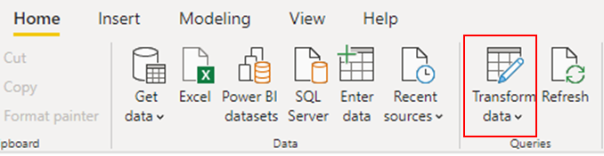
Whenever you need to transform the data, you should use Power Query.
Go to “Home” – “Transform data” to open Power Query.
Let’s begin with the examples! Yay!
We will start with an easy one, okay?! Just to warm up!

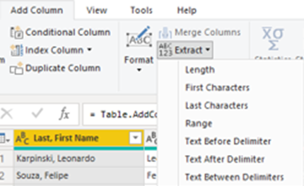
We have a table with one column with the names, and I want to add another one only for the first names. So, I have to add a new column:
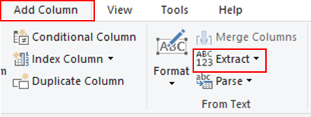
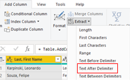
The “Extract” function is to keep the data you want. Then click on “Text After Delimiter”, which in this case is after the space.
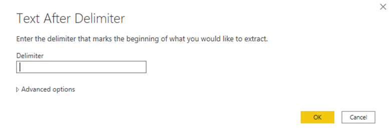
Inside the “Delimiter” blank you click on the space bar, and “ok”.
Once the new column is added, you can see the header as “Text After Delimiter” and rename it.
Just like the example, I renamed it in the formula bar, so there were no steps applied just as shows in “Applied Steps”.
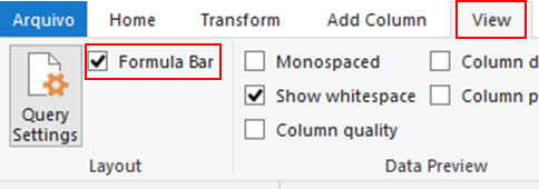
Ah, by the way, you can enable the formula bar if you feel like it’s better.
Now let ‘s make it a little harder. I want to add another column with the first and last name separated only by space. To do so, you have to use the feature “Column From Examples and click on “From Selection”. Then, you give some examples.

Once you give the examples, Power BI assimilates the order and creates a formula to automate.
This feature is a good option to help when you need to standardize words, letters, etc.
Then if your work is done, you click on “Close and Apply”.
Transformation
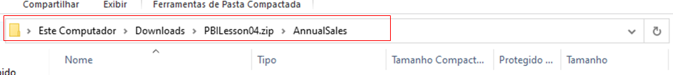
One of the coolest things Power BI allows us to do is to combine information into 1 table. Just like the example, you have a folder with 3 databases in it, and you want to put all the information together.
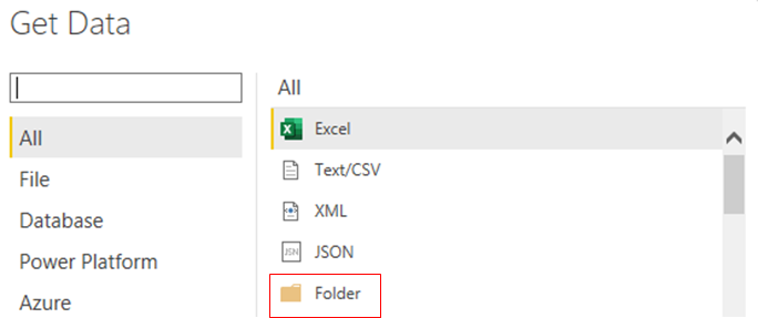
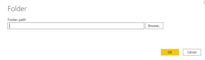
You go to “Home” bar, click on “Get data” and choose “Folder”, then you paste the folder path where the information can be found.
Now let me see if you are really paying attention… What is the first thing to do after choosing the file? You got it right if you said “Transform Data”!!
You can also use the function “Combine file” but I personally don’t like it because your files must have the same name, and it can be prone to error.
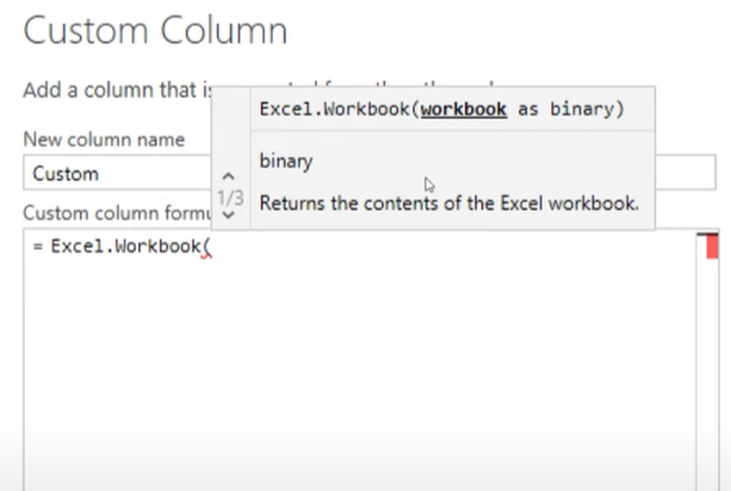
I function I really like to use is “Custom Column”, that connects with a excel workbook, and the formula to do that is what is called “M”. After you adjust and keep the information you need.
Okay, good, first job is done! We combined the tables into one.
I always like to know what are the columns I need at the end of the transformation, which in this case are: year, region, state, city, month and sales.
Then I delete the columns that are empty.
In the “Total” column it must always have numbers. If there is no number, you can remove it. After checking all columns, remove the ones that are empty.
Tip: You never bring totals into Power BI. You must always calculate them in Power BI.
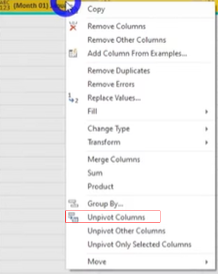
In order to put all the months columns together into rows (lines), I will use the function “Unpivot”. You select the columns you want to work with, and then right-click on any and choose “Unpivot Columns”.
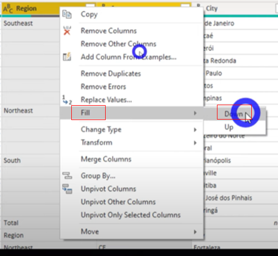
As you could watch in the video, the column “Region” has some “null” lines. To correct this mistake, we have an easy option, but you must be really careful using it, that is to add an intermediate step.
Select the columns you want, right-click and choose the option “Fill” – “Down”
It will open a window asking if you are sure about inserting a step, and if you are pretty sure it is safe to do so, go ahead and “Insert”.
Remember the column we used the unpivot function? Now we will slip it into two columns, one with the month and the other with the number. In order to do so, you know what to do, right? We did it in the begging of the video today.
Let’s see:

Okay, now that we have already extract the “Month”, now in the same column we will adjust:
“Add column” – “Extract” – “Text Between Delimiters”
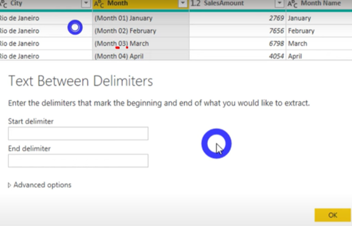
Then change the “ABC123” to “Whole Number”.
All set, “Close and Apply”.
Now to see better what happens when we add another file. Do you think we will need to transform the data one more time?
We have a new file for Sales 2020 that we have to add into Power BI. We will insert this file in the same folder the other ones. Go back to Power BI, “Refresh” and voilà!! We have our chart updated with all files and information!
That was only possible because all files have the same structure!
Now, let’s see another example.
First thing to do once you open the file in Power BI, is to transform the data, right? Remember this golden tip! Then delete the columns and rows I won’t need.
In this example, I’m going to use a new function that is: “Conditional Column”.
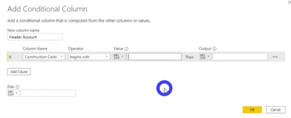
This function is similar to “IF” in Excel.
You indicate the word (Value) to the “Output”.
If an “error” appears, first you have to check why and then replace the “error” by other word. In the example it was “null”.
The second part of the example is using another function. Go to “Add Column” – “Extract” – “Length”. You can see that another column was created, right? In the formula bar, there is a formula for the function we used, copy it because we are going to need later!
Then “Add Column” – “Custom Column”, rename if you need. Now we are going to use the formula we copied into the ‘Custom Column Formula”.
(14 is the number of characters regarding the information we had.)
Once you make all the adjusts, click on “Close and Apply”.
Thus, delete the columns you won’t use, and remove the blank spaces. Also, remember to always (always!) to set the configuration according to the data used in the column, if it’s a text, a number, time, etc.
So, that’s it for today!!
These links below are helpful links to learn more about what we learned today.
https://docs.microsoft.com/en-us/powerquery-m/
https://docs.microsoft.com/pt-br/powerquery-m/excel-workbook
https://docs.microsoft.com/en-us/power-bi/create-reports/desktop-excel-stunning-report
Hope you liked this video and learned more about Power BI!
Don’t forget to like this video and to subscribe!
See you next Thursday!
Cheers,
Leonardo