BLOG DOS
INCOMPARÁVEIS

Hey guys, how are you doing?

Today’s post is about Live # 35, where I talked all about relationships between tables and data modeling. So, follow along and I’m sure I’ll clear up a lot of doubts you have on a daily basis about the topics.

7 Pillars

Within Power BI projects development we have 7 construction pillars:

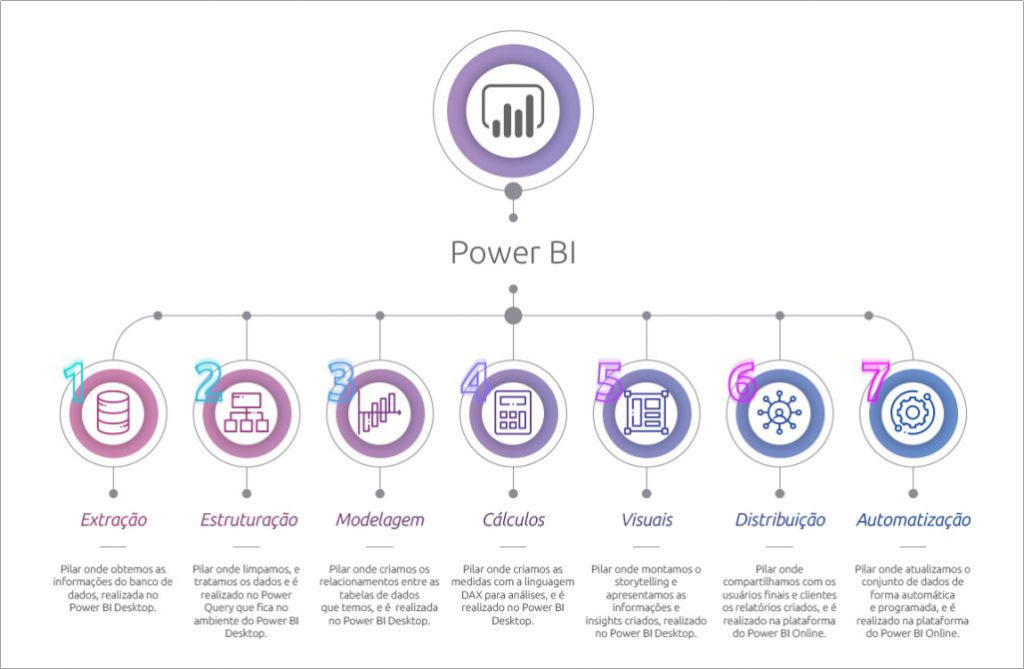
Our focus today will be on the 3rd Pillar! But there is no way to have a good modeling without having a good structure (2nd pillar). So, I want to make it clear to you that these 2 processes are closely linked.

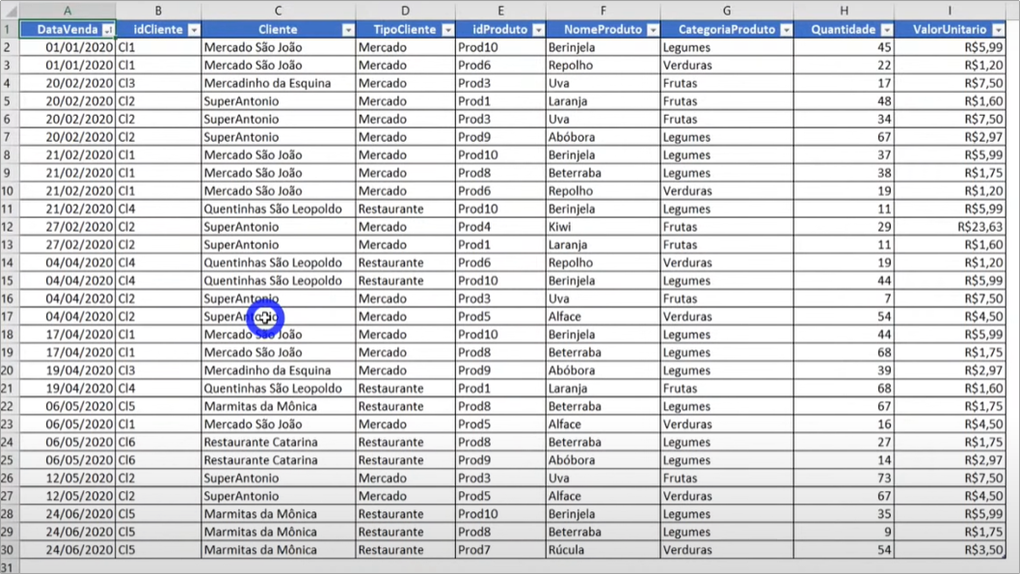
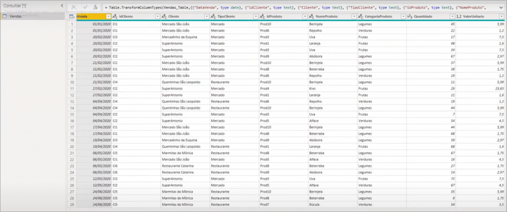
Database – Sales Spreadsheet

For our example, I decided to get the most common database format for those who are starting to work with BI. The famous “big table” … in it, information is usually extracted from a system with several columns (some of them are useless) that can be better structured.

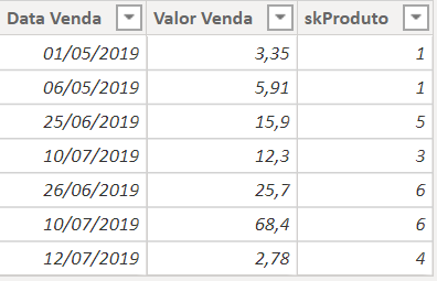
Our first “big table” is a sales spreadsheet for a fictional company:

So, this will be the first spreadsheet from where we will get the data in Power BI:

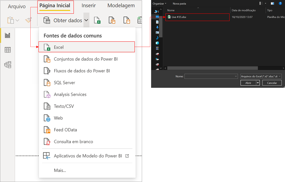
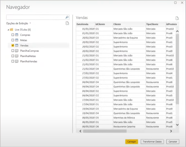
The following screen will appear and you must select the Vendas (Sales) table and click on Transform data:

This step we just performed is Pillar 1 – Extraction, and when we click on “Transform Data” we move on to the Power Query environment where we perform Pillar 2 – Structuring:

In this case, our table is well structured and we don’t need to apply any modification to it.

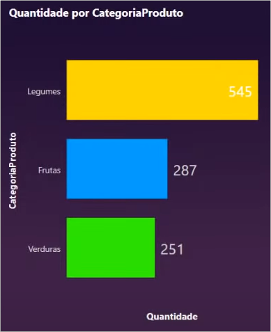
To do an initial analysis, let’s put together a visual demonstrating the amount of sales by product category:

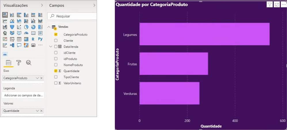
In this case, as we are only working with a “big table”, the sales data are filtered by product category without having to create a relationship because they are in the same table.

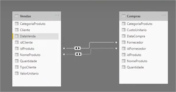
Well, but what if we want to work with both purchasing (compras) and sales (vendas) information? Let’s see what to do …

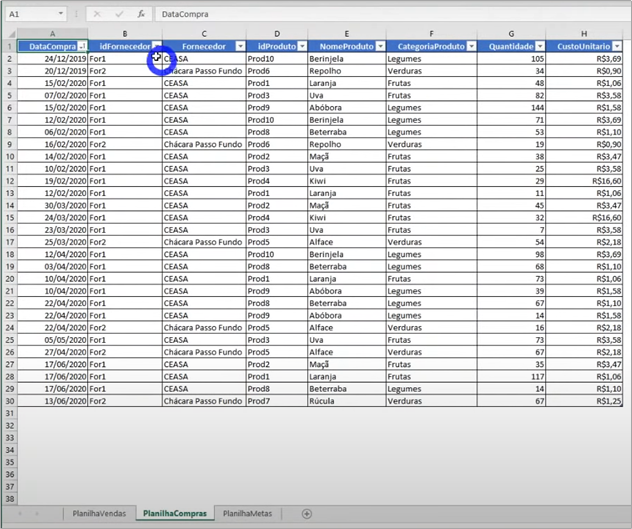
Database – Purchase Spreadsheet

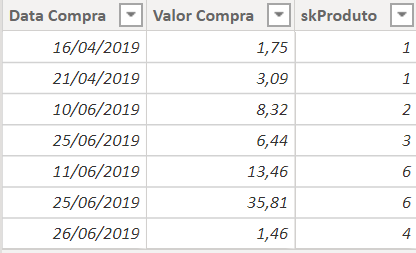
Our purchase (Compras) spreadsheet is in the same file as the sales in .xlsx, but in a different tab.

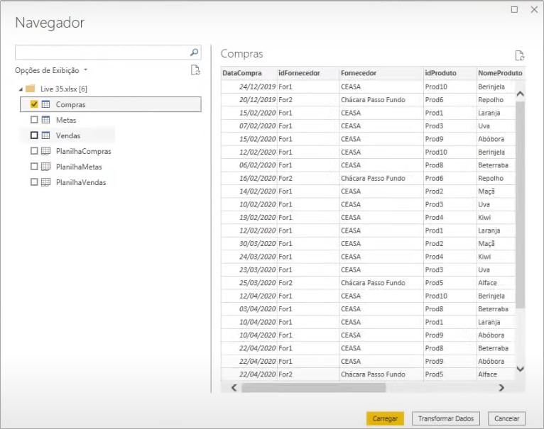
To import it, just do the same steps as for the sales and also select it before transforming data:

In the Power Query environment, we see that this purchases table is also well structured.

So, just as we did for the sales table, we close and apply it in the Power Query editor to return to the Power BI environment.

Relationships

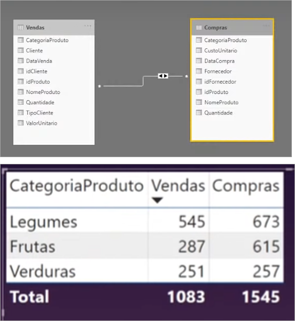
With the two tables imported, we can simulate the relationship between them by assembling a single table where we illustrate the quantity sold and purchased by product category:

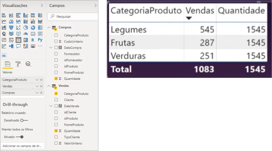
Note that purchase values ​​are not being filtered by product category as well as sales. This is because there is no relationship between the category (categoria) column of the purchase (compras) table and the category column of the sales (vendas) table so the values ​​are equal to the total purchases for all categories.

We can do another simulation, changing the selected sales product category to the purchasing column. Can you imagine what will happen?

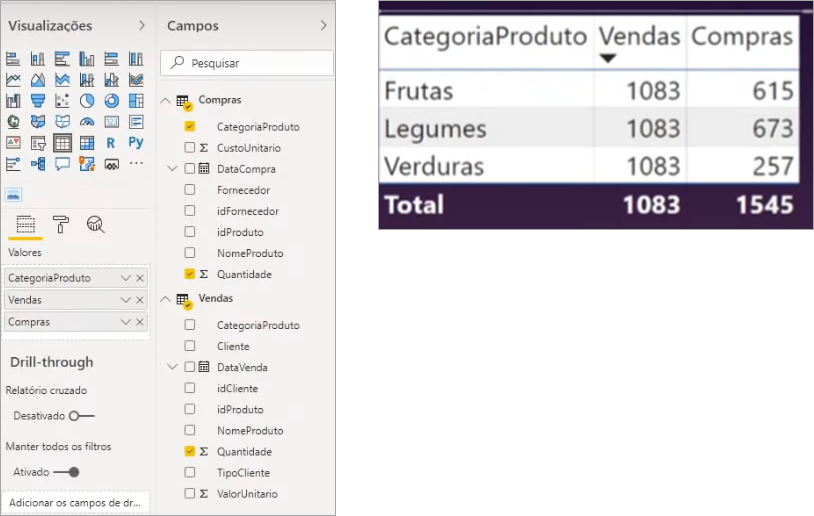
We have already seen that if we try this way, we just throw the problem to the other side.

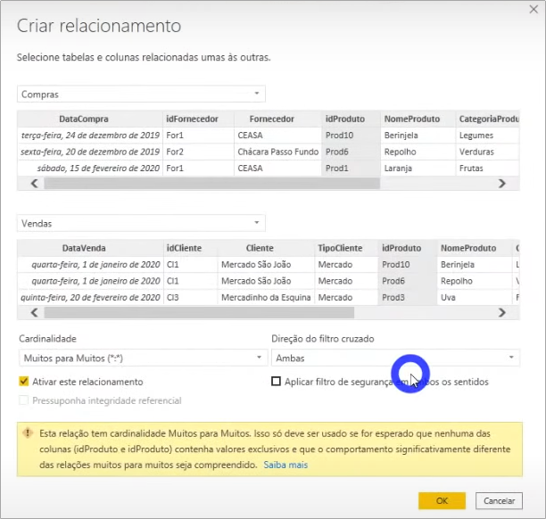
The correct way to work to solve this problem is to use relationships. Opening the “Models” tab, we can see that there is no relationship created between the tables.

In this case, we will create a relationship between the tables by the idProduto column to test what happens:

After creating the relationship, let’s see the table values:

Huh, it looks great! All values ​​in both columns filtered correctly. Now, is this the best way to work ?? Let’s do a test simulating the amount of purchases and sales over time:

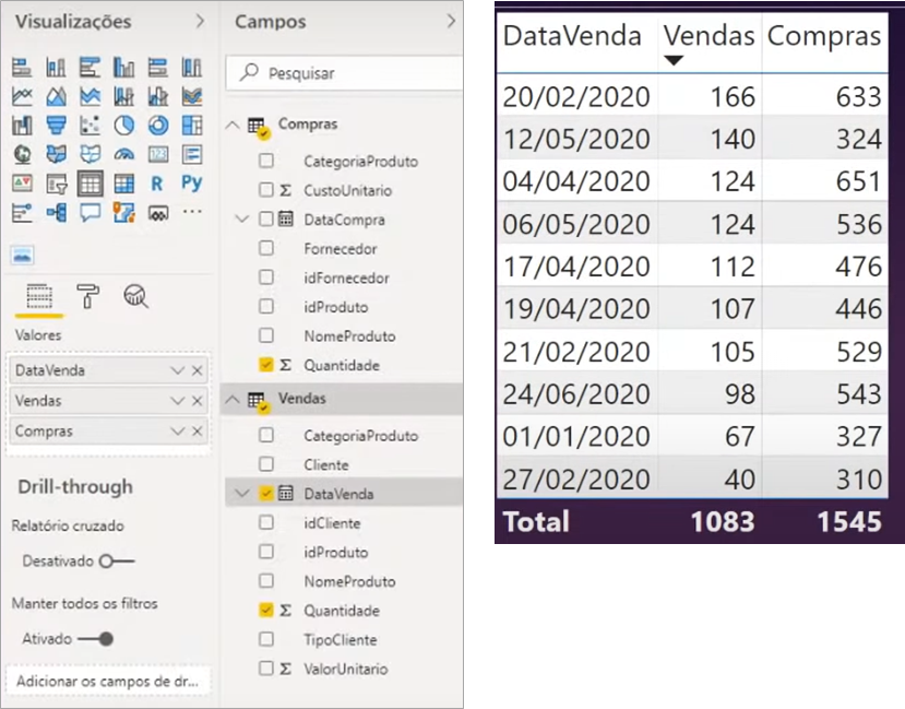
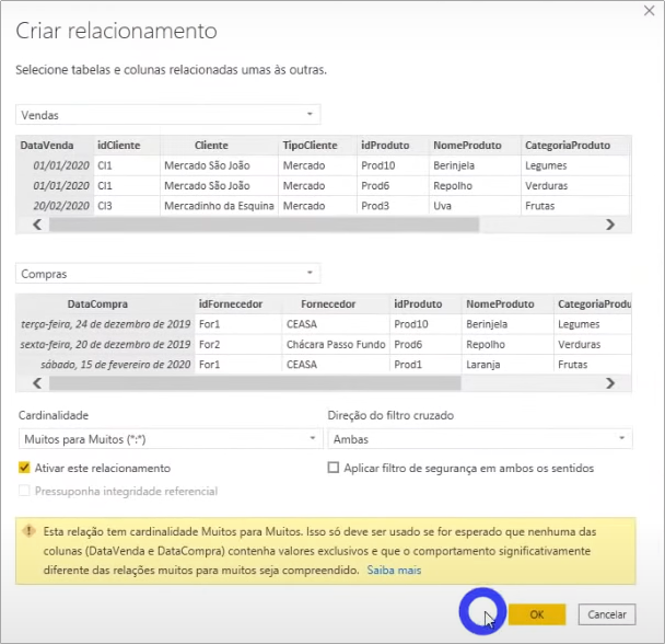
The sales figures seem correct, but what about purchases? In the third line, if we add up, we already have the quantity of 1608, which is greater than the total 1545! We already see here that it’s not correct … Let’s try to make the relationship between the dates columns in our “Model” and see what happens:

The result is:

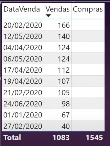
Well, if it was bad before now it got worse because the values aren’t even being displayed. This is because there are dates in wich sales were made but nothing was purchased … So it’s obvious that there will be a purchase amount for that day.

What would be the way out in this case? What if we create the relationship between the two columns (DataVenda and idProduto):

There is no way to maintain 2 active relationships between the same two tables. So, this is not a solution.

The solution for this case is to work with auxiliary tables which are the dimension tables.

Fact and dimension tables

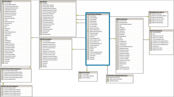
The data is always stored in one or more databases (OLTP). And when I say that, people ask: “What is an OLTP database anyway?”

The OLTP database is a transactional database. It’s where the data is stored in its normalized form, where each information is in a specific table. This way, we have many (a lot) tables involved. And each table has specific information. We call this the normalized model. I’ll show you an example from Adventure Works (fictional company Microsoft created to provide data samples):

Simple? Organized? Yes … generally, the database is not as organized. In this format, for those who work with OLTP database, this is very well structured!

For those who don’t have a lot of knowledge about the subject, when getting a database like this, don’t know for sure or how to start. And preferably, when we work with Power BI we should access another middle layer which is called DataWarehouse (DW).

In it the scheme is more simplified with fact and dimension table structures. The result would be something like this:

This way, the connection becomes simpler and more performance-oriented to work. In reality, DataWarehouse is not always used, and many people connect directly to the transactional database (OLTP), which poses risks to the information flow.

Our goal is to create a model using the denormalization process. Putting all the information together in a single table. This is not the best way to work with, but it’s very realistic. The best way to work with is the dimensional model with fact and dimension tables). The definition of these tables is:

– Dimension table: it’s a table that has information related to some business entity (some item registering)
              – It’s mandatory to have a unique ID (code / primary key) that represents the dimension

– Fact table: it is a table that has movements, events / historical records (usually has a date related)
              – What do I need in the Fact Table that is relative to the dimension? Dimension ID (ID) only

Creation of fact and dimension tables

Let’s create our fact and dimension tables from scratch. It all starts with checking what the dimensions are in your model, and that requires a good deal of time to carefully analyzing your data.

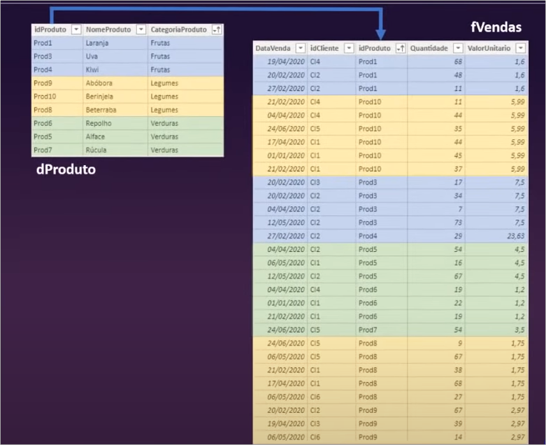
In our example, the dimension tables are:

• dCliente with the columns: ID Cliente, Cliente e Tipo do Cliente
• dProduto with the columnss: idProduto, NomeProduto e CategoriaProduto

To create the dimension tables we use Power Query as the main tool. In it we will merge the two fact tables, remove the unnecessary columns in our dimensions and also remove duplicate information.

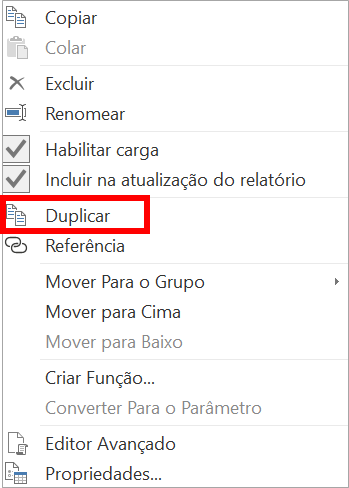
Right-click on the Sales table and select Duplicate (Duplicar on the image below):

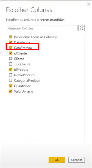
Let’s call this new query dCliente (double-click it to rename it). Next, we must choose which columns will remain in that table (only customer-related columns):

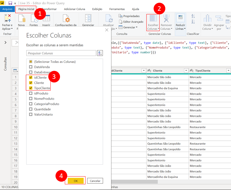
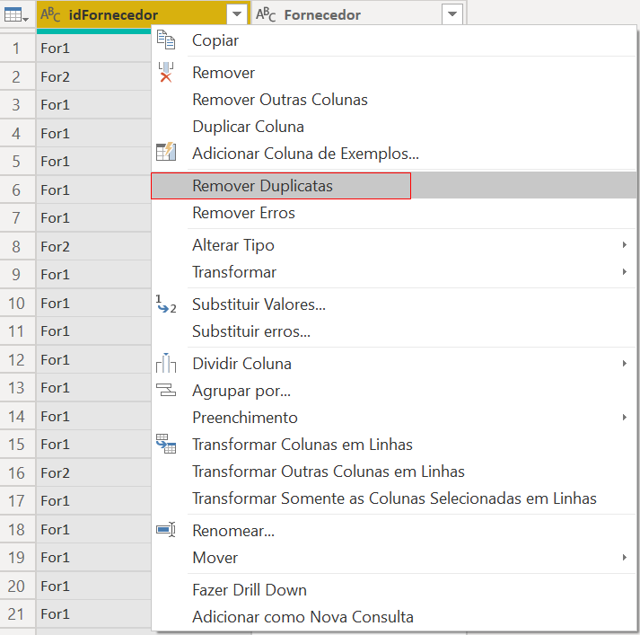
You should now remove duplicates from the dCliente table. To do this, just right-click on the idCliente column and select “Remove Duplicates”. Ready! We have the dimension table for customers.

To obtain a dimension table for suppliers you must do the same thing, however, you will now need to duplicate the Purchasing table (fCompras).

Repeat the same steps, but this time you need to keep only the idFornecedor (Supplier ID) and Fornecedor (Supplier) columns. This duplicate query will be called dFornecedor, so rename it. Also, remember to remove duplicates based on the Supplier ID column, okay?

To obtain the dProduto table, we will need to do it a little differently since both tables (Vendas and Compras) have product data.

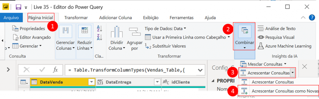
Duplicate the fVendas table first, and then Duplicate. The first will be called dProdutoVendas and the second will be called dProdutoCompras. Remove all columns that are not related to Product, that is, leave only idProduto, NomeProduto (Product name) and Categoria produto (product category) with the “Choose columns” feature we had used before. Now, go to Home → Combine → Append Queries button arrow → Append Queries as New:

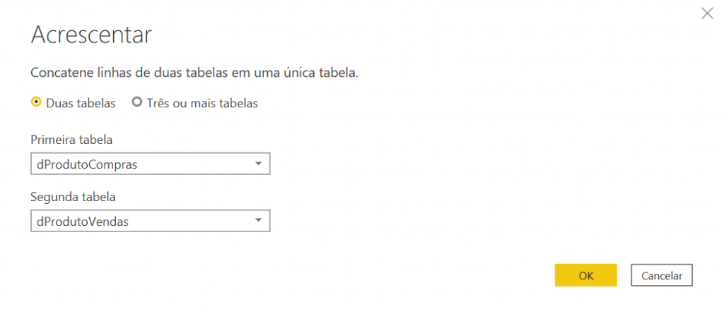
If you are in the dProdutoCompras table, the second table will be dProdutoVendas, otherwise, do the opposite. Just select the second table according to the image below:

Finally, in this new query, right-click the idProduto column and select “Remove duplicates”. Ah, call this query dProduto.

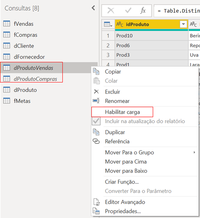
As we will not need the queries dProdutoVendas and dProdutoCompras, we can disable their load. Just right-click on the query and deselect “Enable load”. In the end, both tables will have the name in italics, like this:

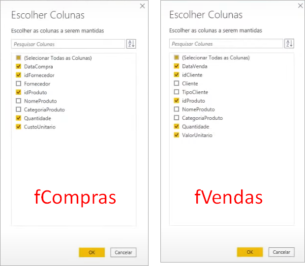
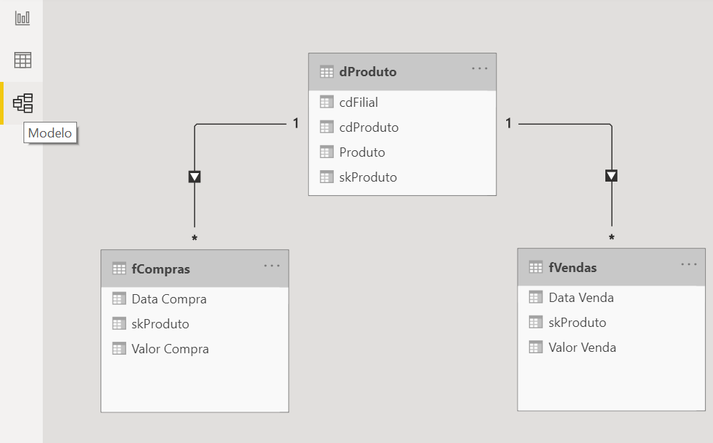
With the dimension tables ready, we rename our fact tables with the prefix f (fVendas, and fCompras).

Now to finish, we remove the unnecessary columns from our fact tables leaving only the columns with the primary key to connect to the dimension tables:

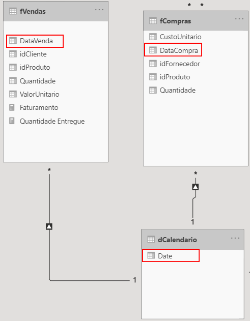
Alright, with that done we have our fact and dimension tables completed! Now let’s create our relationships in the model.

Creating relationships

When we go back to the Power BI environment after clicking “Close and Apply” some relationships are built automatically. In our case, we will exclude all of them as well as the ones we had created to build everything from scratch. Click on each link (connection between the tables) and press “delete” on the keyboard.

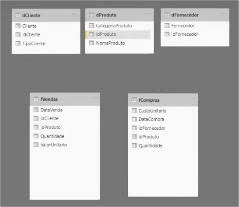
After deleting all of them, let’s create the new ones as follow: drag the column name from one table towards the other. List of relationships:

• dFornecedor with fCompras: through idFornecedor
• dCliente with fVendas: through idCliente
• dProduto with fCompras: through idProduto
• dProduto with fVendas: through idProduto

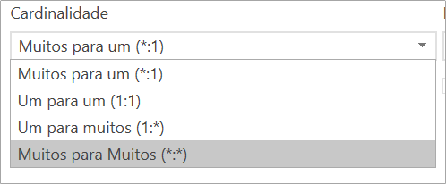
See that there is a format at the end of each table in the row where it shows the relationship between them (they are the 1 and *). This illustrates the cardinality of this relationship. Cardinality explains the way in which those tables are related, and there are 3 types:

1. One to many (1: ) or many to one (: 1): there is a single row in table 1 that relates to several rows in table 2 (for example: a single row of our Product id with multiple rows that have Product id in fCompras)
2. One to One (1: 1): a row in table 1 relates only to a row in table 2
3. Many to many (*: *): several rows in table 1 relate to several rows in table 2 (this case is very dangerous because it can cause a performance issue and ambiguity in your project)

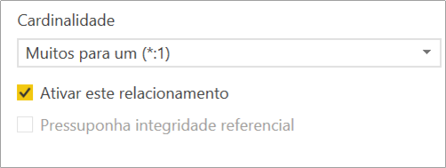
Another characteristic of the relationship is whether or not it’s active, if it isn’t active, the relationship won’t result in the creation of evaluation contexts for its tables. There are cases where you can activate the relationship that is inactive through the USERELATIONSHIP function to an extent:

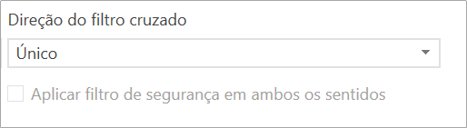
And finally, we have the direction property of the relationship that can be in both directions (that is, the tables can filter both from table 1 to table 2 and from table 2 to table 1). The shape of both directions doesn’t appear often (I guess less than 1% of cases) and should be avoided in the models as it can cause ambiguity. In general, we use the single filter direction:

With that, we have the explanation of each attribute of the relationships as well as all of them created and we can move on to the examples.

Application example

The first example we are going to do is exactly the same bar chart we did previously for the amount of sales by product category. The difference is that in this case the category column comes from the dProduto table and not from fVendas:

The result looks good and matches what we had previously done! We can understand the applied relationship as a filter that propagates from the selection made in the dProduto table to the fVendas table. Visually it would look like this:

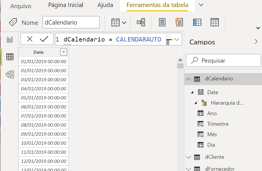
Creating the dClendario (Calendar) table

In addition to the dimension tables we create based on the fact tables, we have another dimension table that we use to make the relationship between dates. This table is commonly called dCalendario. Go to Modeling and click on the following button to create a new table:

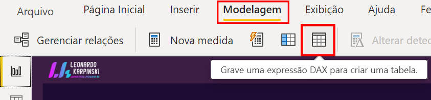
DAX Formula:

dCalendario =
CALENDARAUTO

And with the created dCalendario, we make a relationship with both fVendas and fCompras:

Now, I have the dCalendario table related to the two fact tables so we can make the analysis over time of the two tables in a visual:

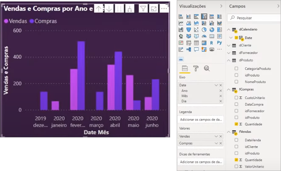
So, with the support of dCalendar table we can do this kind of analysis between 2 or more fact tables.

Relationship scheme

There are some relationship schemes. The main one that should be preferably used is the Star Schema where the fact tables are related only to dimension tables and dimension tables are only related to facts. Another well-known model is Snow Flake, where there are cases where dimension tables have relationships with other dimension tables. It is a known type that is also used, but it has worse performance and greater difficulty in creating hierarchies.

Granularity

Imagine now that you have to evaluate the results compared to the goals but the table of goals (Meta) has a result by product category (you must remember that in fact we have the idProduto). In this case, we have a different granularity between the tables.

See our base of goals below:

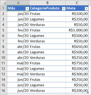
Let’s import our goals ((Metas) table from the same base Excel file:

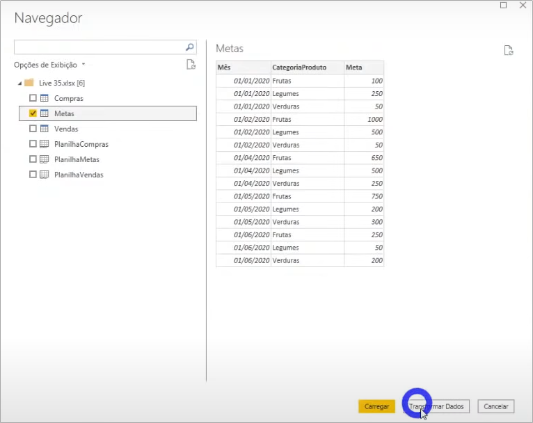
The goal table is a fact table that has not yet occurred, but is expected to occur. Another way to think about whether or not it could be a fact table is to analyze the columns it contains. Realize that it has both date (mês) and product (CategoriaProduto) information. This way, we already have a very good indication that it’s a fact table. So, let’s rename: in Name in the query properties, type fMetas.

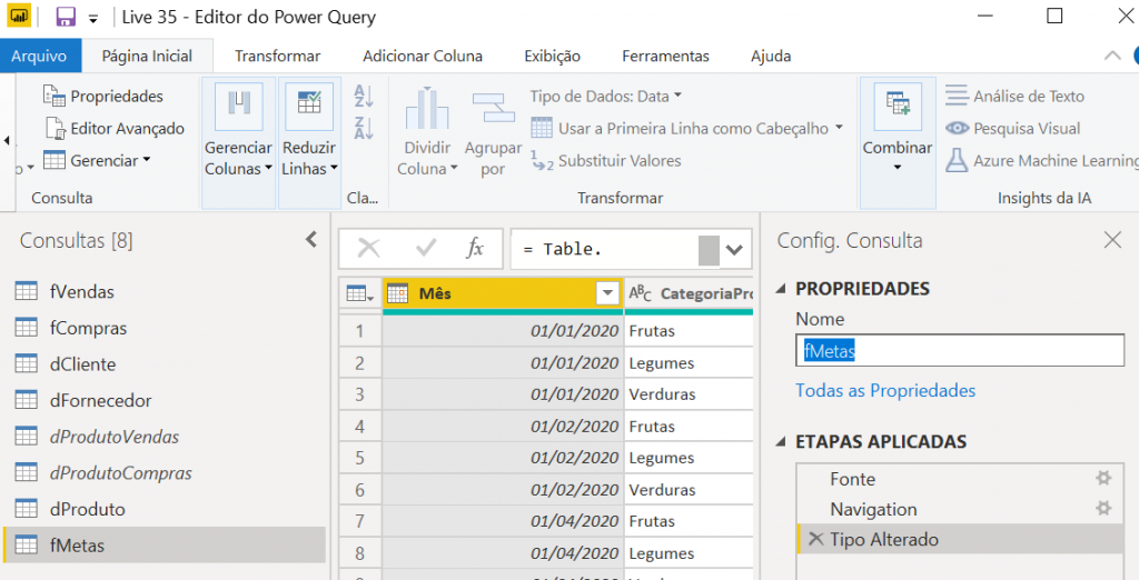
Now, we can close and apply to go back to the Power BI environment to create the relationship for this table – which is where the biggest challenge is.

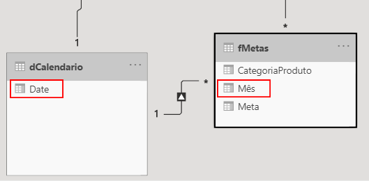
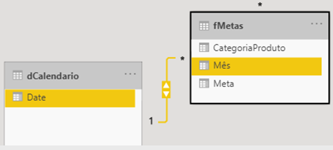
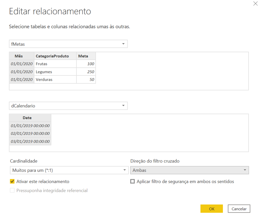
It was easy for the relationship between fMetas and dCalendario, as Power BI automatically changed the month to the start date of that month.

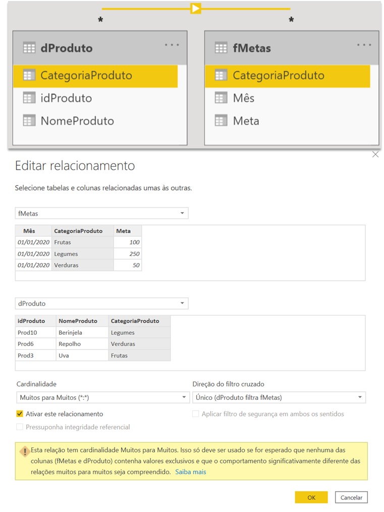
Now, for the relationship between dProduto and fMetas, we have to be very careful in the direction of the filter that we will keep selected as this can cause errors in your report. In this case, always keep the direction of the dimension table towards the fact table:

To measure sales compared to the goal, let’s create a Revenue (Faturamento) measure:

Measure:

Faturamento =
SUMX ( fVendas, fVendas[Quantidade] * fVendas[ValorUnitario] )

Now, we can compare side by side in a matrix how much we have as revenue compared to the stipulated goal:

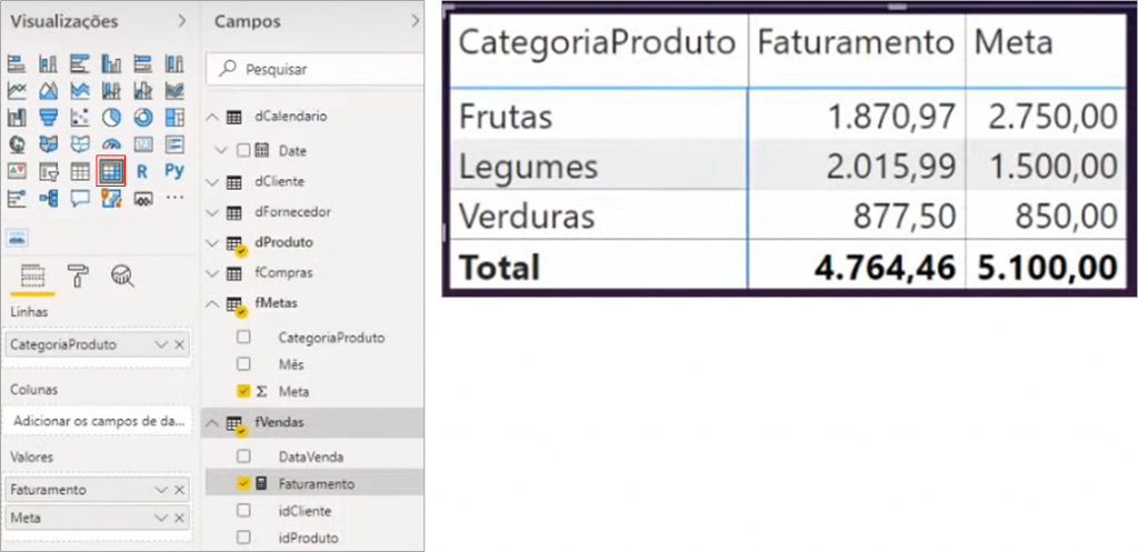
So far so good, the problem occurs when we want to go down to the product level. See how it looks when we add this hierarchy (by dragging ProductName to the Visual lines field):

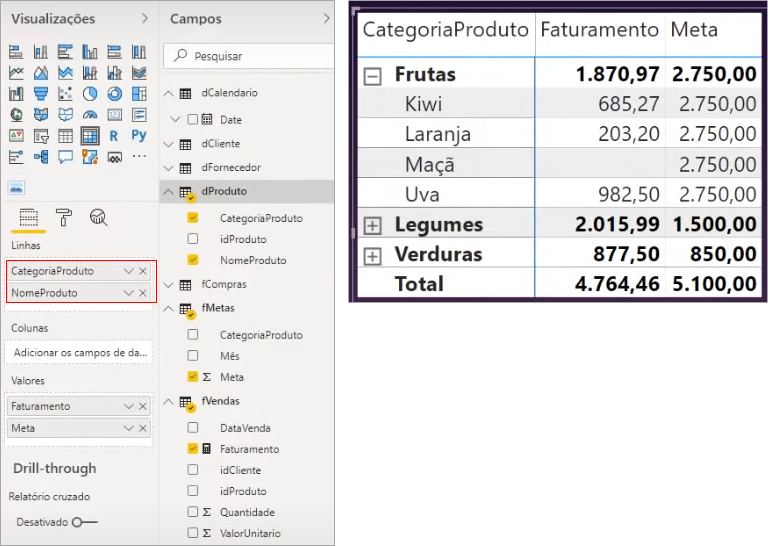
In this case, the goal remained the same within the sub-level and to correct this we have to create a business rule, for example, divide the total value of the category for each of the products.

Single and Both-Directional Relationship

As I said earlier, it is very risky to use a relationship for both sides, as the problem of ambiguity can occur. One way to analyze if you can have this problem is to try to reach the same table from a base table by more than one path following the the relationships created flow.

Let’s go to an example where I modify the relationship between fMetas and dCalendario for both-directional:

See the configuration of this relationship:

Power BI has an intelligence that forces the use of the shortest path in this type of analysis. However, I strongly recommend that you do not use the relationship in both directions, because for more specific cases we have the option of using the CROSSFILTER function in DAX that forces this type of relationship virtually. So, go back to the previous filter status (Single), ok ?!

Inactive relationship

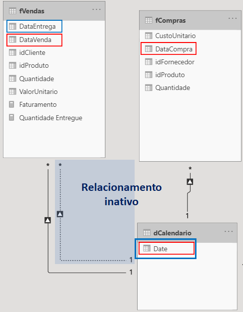
To simulate the inactive relationship, we need to have two columns from the fact table that relate to the dimension table. Here, I will create a delivery column in the fVendas table in addition to having the relationship between the sale date with dCalendario and also having a relationship between the delivery (DataEntrega) column (which will be inactive) and the dCalendario table:

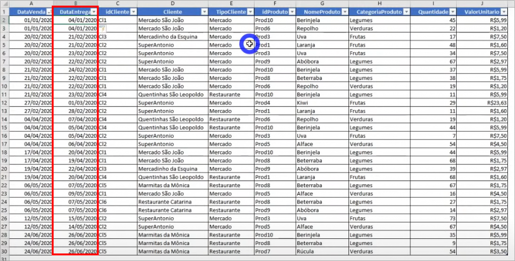
Remember to change that fVendas column selection step:

Now, relate the DataEntrega to Date, and see that the connection will be dashed:

This way, you can make an analysis based on the product delivery date. However, we need to discriminate this as it will do the calculation because it isn’t the default (active). Let’s create a measure with this characteristic:

Measure:

Quantidade Entregue =
CALCULATE (
    SUM ( Vendas[Quantidade] ),
    USERELATIONSHIP ( fVendas[DataEntrega], dCalendario[Date] )
)

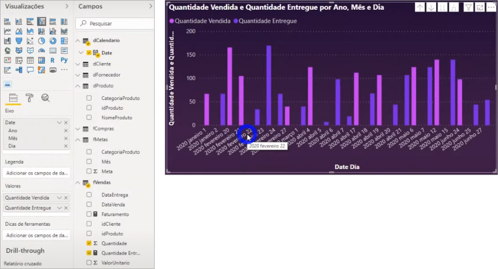
With the created measure, we can analyze in the same visual the quantity sold and delivered of products for each date:

Composite key

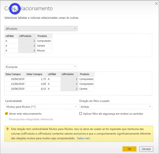
There are cases where the same code can represent different things within the company (for example, in a company with branches the same material register id can be used for completely different materials). In these cases, we have two options:

1. Concatenate: create a unique code by concatenating the column values
2. Surrogate key: it’s the most elegant way where you create a key (I’ll do the example with you)

If you don’t do any of the options when trying to create the relationship in Power BI it will inform a relationship from many to many:

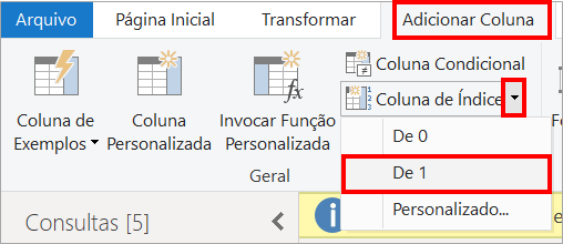
The first step in creating the surrogate key is to create an index column in Power Query:

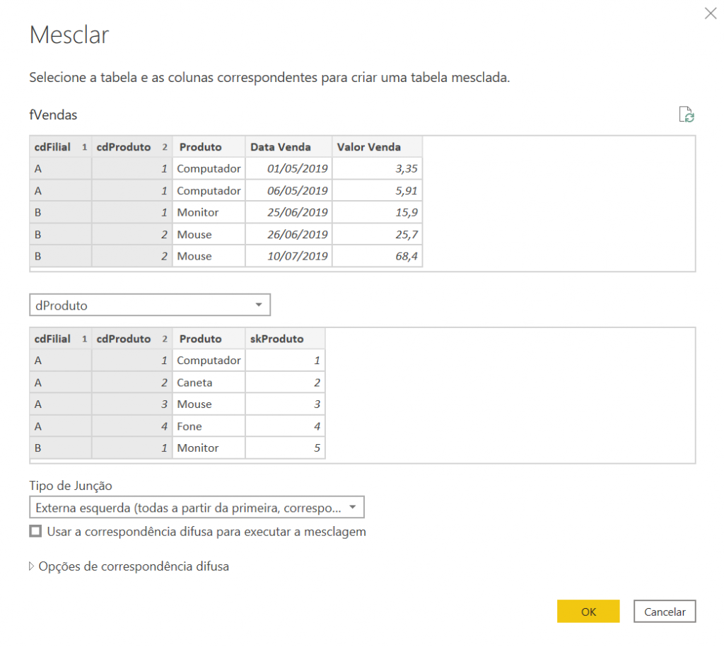
This way, we already have the unique key in dProduto. And how to make the connection with fVendas? By merging the queries and selecting the two columns that uniquely identify the product:

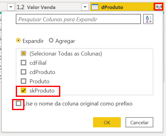
After that, we expand only the column with the information of the surrogate key:

Having this information in the sales table, we can delete the other columns with product information from the table:

And doing the same process for the purchase table we have the result:

We can close and apply, and Power BI will automatically create the relationships between the tables that we can see in “Model”:

Well guys, here in this definitive guide I covered several examples people have may encounter in the real routine when working with relationships in Power BI! I hope it helped you and if you have any comments or questions leave them below.

Regards,
Leonardo.