Hey everyone!
Have you ever needed to make annual or monthly comparisons on billing, number of customers, products, etc.? Calculate some of these values on an over the year accumulated figure? Or even calculate any value that depends on any time variable (month, year, day)? If so, you can’t miss today’s content because we’ll talk about DAX Time Intelligence functions. There are several functions ready to facilitate aggregations over time and you will see how practical and easy it is to use them!
Before starting, I will indicate two sources for DAX functions: Official Power Bi Documentation, and Dax.Guide.
Scenario Description
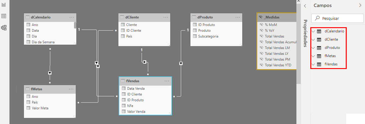
We have a scenario with the following tables: dCalendario, dCliente, dProduto, fMetas, fVendas.
In today’s content, we will focus on the DAX Language, so the import, transformation, and data loading steps will be explained in another post, okay?
Let’s assume that we already have the Total Sales measure.
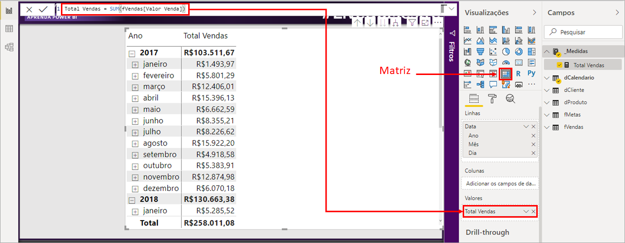
Formula:
Total Vendas = SUM(fVendas[Valor Venda])
We will also select a matrix visual so we can visualize the measures we will create from now on. On the matrix visual will insert the Date field in the rows and the Total Sales measure in the column. Check the image below:
Annual accumulated – Year To Date
Annual accumulated with DATESYTD
We are going to create a measure to calculate the cumulative Total Sales (Total Vendas in portuguese) for a given period. Check below:
Formula:
Total Vendas YTD =
CALCULATE(
[Total Vendas],
DATESYTD( dCalendario[Data] )
)
DATESYTD: Returns all dates of the year, from the first day to the maximum value of the ‘date’ (day, month, year) of the context.
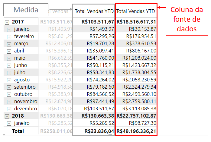
After changing the measure format to Currency, editing the number of decimal places to 2, and adding it to our matrix, we will have the following result:

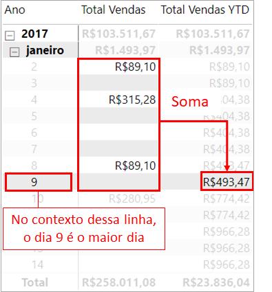
Note that the sum of the first three months of the Total Vendas column is equal to the value of the third month (March) of the Total Vendas YTD column. So, what this measure is doing is accumulating the values from the first day of the year to the maximum day in the context (in this example March).
Drilling down to also display the days, you can see how the Total Sales column looks and how the calculation is performed internally:
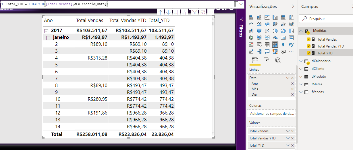
Note that there is a function that also returns the same value as the measure we’ve just created. Check below:
Formula:
Tota Vendas YTD =
TOTALYTD(
[Total Vendas],
 dCalendario[Data] )
)
You can see that it resulted in the same value we had found before:
Personally, I don’t like to use it because it hides what’s behind it (which is the use of CALCULATE and DATESYTD). Besides, using the first version (with CALCULATE) I could state filters as an argument, while in the version using TOTALYTD this isn’t possible
Well, can’t I bring the Total Vendas YTD calculation straight from my database?
Yes, you can. We’ll show you a frequent problem you may face when you choosing to do so.
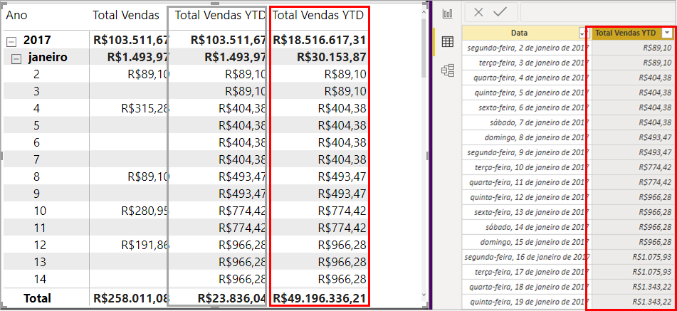
Let’s assume that we bring this Total Vendas YTD value already calculated from the database. Adding this column in the matrix, comparing the column we had calculated previously (measure) with the column imported from our data source:
See that the values don’t match in the image above (when we look at the matrix in monthly granularity). Note that when we drag the imported column into the matrix, the sum of the days (from that same column) was performed.
Also note that when drilling down to display the days (daily granularity), the two columns present the same values (because there is no level after days – time, for example):
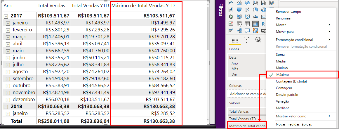
See that when we drag a column into a visual, Power BI already configures that column to sum the values. We could then configure this column to obtain the maximum value, right ?! Let’s do this! Right-click in the (Visual Values) column and change from Sum to Maximum. Note that the measure and column values are now the same, but the total line (the last one in the matrix) is still wrong.
Another issue when we bringing columns already calculated from our database is that when applying, for example, a Country filter, the column will not respect that external filter. Note that when we filter any country, the Maximum Total Vendas YTD column will remain unchanged while the column with our Total Vendas YTD measure will consider the filter applied correctly.
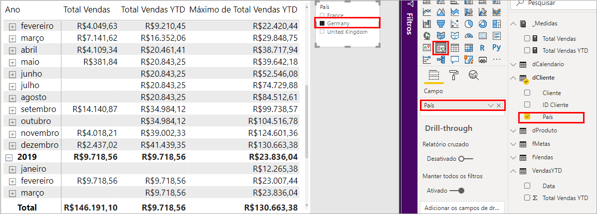
Important:
The biggest issue with bringing “ready” calculations from the data source is related to granularity (analysis level) and filter (values are static).
Let’s move on to our next measure!
Monthly variation (% MoM)
Now our goal is to calculate the change in the Sales value compared to last month (month over month). In other words, we need two pieces of information: the previous month’s value and the current month value (current context).
Last Month with DATEADD
Whenever we want to create a measure with DAX we must keep in mind that all the values it uses must be visible in the context. This means, if we want to calculate the monthly variation, we need to bring the previous month’s values to the same line (context) where we are calculating this variation. What we need to do first is bring that past value into the ‘present’ context. We will use the DATEADD function as below:
Formula:
Total Vendas LM =
CALCULATE (
[Total Vendas], DATEADD ( dCalendario[Data], -1, MONTH ) )
DATEADD: It is very useful for calculating the percentage of growth over time. It is used to move forward or backward in time (years, months, days, etc.).
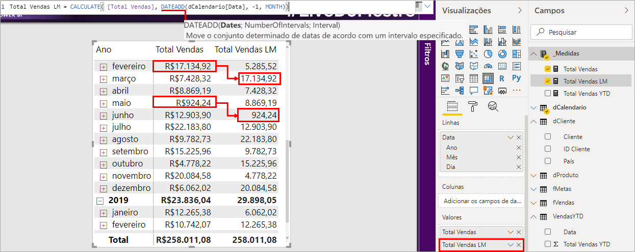
See that in the image above the Total Vendas for February was moved to the line of March (we moved back 1 month in context) as well as the Total Vendas for May was moved to the line for the of June in the column Total Vendas LM.
% MoM with DIVIDE
Now, let’s calculate the monthly variation (month over month) using the DIVIDE function. Since we want to determine the variation, we need to calculate the difference between the two values and then divide that difference by the last one. Check the syntax below:
Formula:
% MoM =
DIVIDE(
    [Total Vendas] - [Total Vendas LM],
    [Total Vendas LM]
)
DIVIDE: It’s used to divide two values. The difference between using it instead of the divide (/) function is that when using DIVIDE, if the denominator is zero, then by default the resulting value will be Blank (empty) unless you specify another value in the third argument of the function.
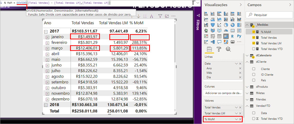
Note that in the matrix shown in the above image, the column with the measure % MoM is blank (Blank). Remember that the DIVIDE syntax asks for 3 arguments? Since we didn’t specify anything in the third argument, it defaults to Empty. Looking at the March line of the matrix, the calculation was performed correctly.
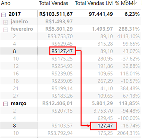
DATEADD considers the full period (in this case: month) or the context?
Youtube Live Participant
It considers the context. See that Total Vendas LM resulted in the value of Total Sales for February 8 (1 month back exactly). See the image below:
If we wanted to repeat the value of Total Vendas for January on every line (days) of the following month, we could use the PREVIOUSMONTH function. Check the syntax:
Formula:
Total Vendas PM =
CALCULATE(
    [Total Vendas],
    PREVIOUSMONTH ( dCalendario[Data] )
)
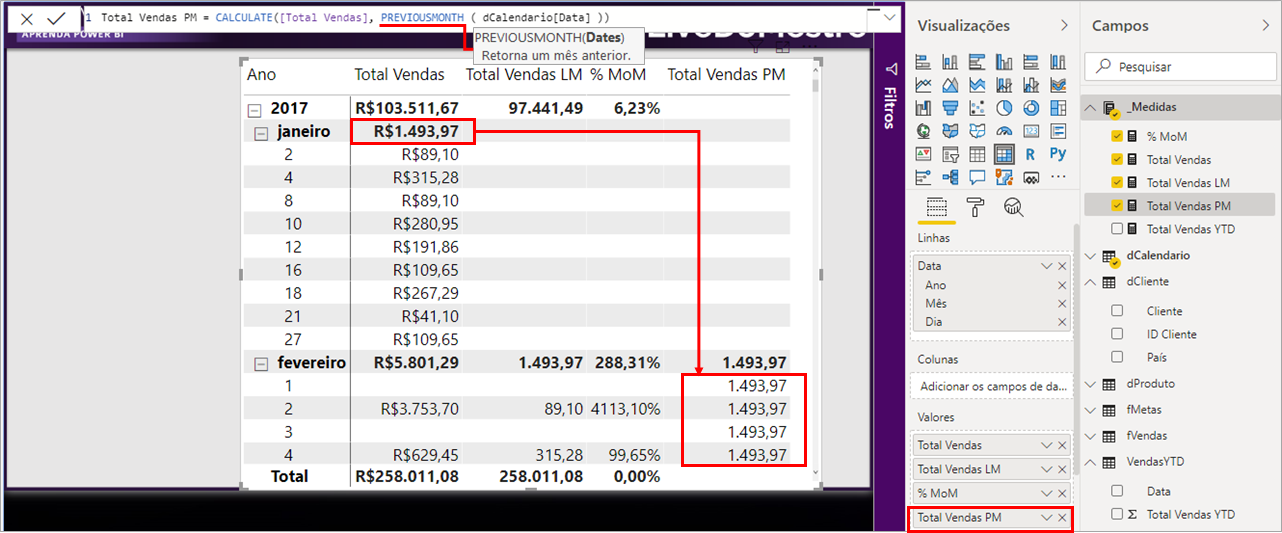
Note that we were able to obtain Total Vendas for January across all February context lines in the Total Vendas PM column.
Annual Variation (% YoY)
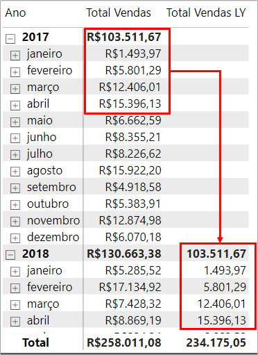
Similar to what we did with months, let’s find the previous year’s Total Sales:
Formula:
Total Vendas LY =
CALCULATE(
    [Total Vendas],
    SAMEPERIODLASTYEAR( dCalendario[Data] )
    // DATEADD( dCalendario[Data]; -1; YEAR)
)
Note that this time we used the SAMEPERIODLASTYEAR function. If we used DATEADD as commented (read the line after the two // bars), we would have the same result. We use DATEADD in the Total Vendas LY measure because there is no similar function (yet) for months, ok ?!
Accumulated value
If we needed to accumulate values from the first to last Sales day, how could we do that? Unfortunately, there is no out of the box function for this, so let’s create the following measure and use variables to help us:
Formula:
/*Option 1: without using the FILTER function */
Total Vendas Acmuladas =
VAR vLastDayContext = MAX(dCalendario[Data])
VAR vAccumulated =
CALCULATE(
    [Total Vendas],
        ALL(dCalendario),
        dCalendario[Data] <= vLastDayContext
    )
)
RETURN
vAccumulated

/*Option 2: using the Filter function */
Total Vendas Acumuladas =
VAR vLastDayContext = MAX(dCalendario[Data])
VAR vAccumulated =
CALCULATE(
    [Total Vendas],
    FILTER(
        ALL(dCalendario),
        dCalendario[Data] <= vLastDayContext
    )
)
RETURN
vAccumulated
The ALL function returns the entire Date table in the dCalendario table, right? We also know that we have to sum the sales value so that this sum stops only on the last day of that context. Therefore, we use the variable vLastDayConext! Alongside the FILTER function, it will be possible to sum [Total Sales] so that this sum “stops” in each specified context (without the need to restart from zero).
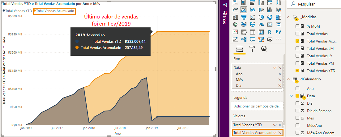
Our goal was to keep the accumulated calculation even after turning to the next year. See, that our previous measure (Total Vendas YTD) has a saw shape – the value is accumulated from the first day of January until the last day of December for each year when the curve falls – note that in the following year, this value starts from zero … With this new measure (Total Vendas Acumuladas), we were able to accumulate the values from the first day to the last of each context. See the comparison of the two measures graphically (in Feb / 2019 we had our last sale – constant value from that date):
What if we want to accumulate the values per product?
Youtube Live Participant
We already made a video on how to build a Pareto chart (we calculate the accumulated value per product there). Click here to view.
Well, now we are ready for our challenge!
#Challenge: Churn MRR YTD
In this challenge, we will answer the following question: how much will I fail to earn due to the loss of customers who canceled a contract with my company ?! What is the total amount of this loss at the end of the year ?! The goal is to calculate the Churn MRR YTD.
Tip:
Churn is the amount lost in terms of customers who left the company (they canceled the contract);
MRR (Monthly Recurring Revenue) is a type of recurring revenue. Ex: If you have customers who sign a contract (lasting n months) with your company and in return, you provide some service, this revenue can be called MRR
Let’s check in Excel the main idea of what we need to do with DAX:
Let’s assume that we had these revenue loss values in column B. How should we estimate what the accumulated annual revenue loss would be (in December), which means, what value are we failing to gain from the loss of these customers (revenues or contracts) until the end of the year?
We will create the following measure:
Formula:
Churn MRR YTD v2 =
VAR MonthContext = MAX(dCalendario[Mês])
VAR YearProjection =
SUMX(
DATESYTD(dCalendario[Data]), //For each month context I need to scan again from the beginning of the year, until the last day of the context
VAR MonthIteration = CALCULATE(MAX(dCalendario[Mês]))
RETURN
[Churn] * (MonthContext - MonthIteration + 1)
)
RETURN
YearProjection
The logic we must keep in mind is: looking at the revenue loss in Jan / 2019, we need to accumulate ‘that loss’ in 12 months; the value for Feb / 2019 in 11 months; March in 10 months, and so on (see Excel formula for help). So imagine that we are in line with the context of Mar / 2019 (remember that in March I need to accumulate the amount for the following 10 months?): The formula should provide us the accumulated of 12 months – 3 months + 1. It is exactly what the MonthContext – MonthIteration + 1 part of the formula shows.
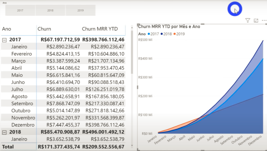
Check how our solution looks now:
Look at the March line! Until March we know how much loss we had, right? We just have to accumulate the Churn values from Jan and Mar: see the use of the function we learned today, DATESYTD. Now, to know the next values (of the lines where the Churn column is empty), we also need an iterator variable: MonthIteration. To fully understand this solution I suggest that you ‘date’ this formula a lot! It is not easy to understand at the beginning, ok ?!
See how nice the chart was when we analyzed the 3 years (removing the year filter = 2019 that was applied in the previous image)… Note that the value of “loss” of revenue grows over time in an almost exponential way. This is the importance of analyzing the loss of customers from an accumulated perspective!
Incomplete periods comparison
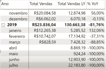
Now, let’s solve a question: how to compare values of incomplete periods (years). We have a column with Total Vendas and Total Vendas LY (referring to the previous year). In the bold line of the matrix, we have two non-comparable values (since one represents the sales value of 3 months from 2019, while the other represents the sales value of 12 months of the previous year, which means, the year is complete). Consequently, the calculation of% YoY is much smaller, see below:
Our solution will be to create a calculated column in dCalendario checking whether or not there are sales, see:
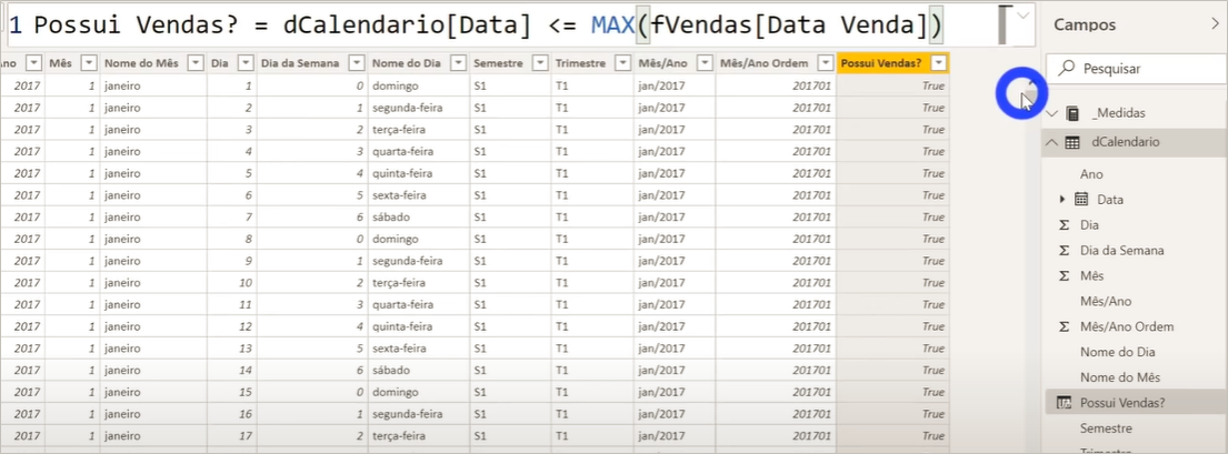
Formula:
Are there sales? = dCalendario[Data] <= Max(fVendas[Data Venda])
See that this formula is Boolean, which means, it already returns True or False. Now just use this column in the Side Filter (Visual) and check the option “True”.
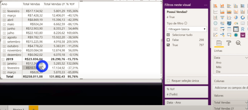
See how simple it is ?! Now we will have no more problems with future dates without sales in our visual and consequently incomplete years’ values being compared inappropriately!
Well guys, this was our content today based on Live # 2! I hope it was useful!
Regards,
Leonardo.