BLOG DOS
INCOMPARÁVEIS

Hey guys! How are you doing?!

Wish to increase your knowledge arsenal about DAX? Do you seek to stop creating workarounds for numerical set intersections? I will show you examples of real application for each of these functions: CALCULATETABLE, INTERSECT, EXCEPT, TREATAS, IN, and much more!

An important note: Today’s content is for those at intermediate to advanced levels in Power BI, ok ?! That is, you already need to know what a calculate function does, for example. If you need to remember, take a look at this material.

Objectives

Do you remember the 7 pillars for building BI projects?

The focus of today’s content will be on Calculations using DAX measures.

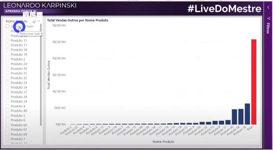
A lot of people make workarounds in order to show the Total value alongside with other values ​​(sales by product, for example) on the same graph. I will show you how to do this by using some specific functions. More than that, I will also teach you how to present the category “Others” when a filter is applied to a visual. This way, in a bar chart, for example, we will have the selected products, the category “Others” and the Total. See a Spoiler of what we will do:

We’ll also create measures to calculate the number of recurring, new and lost customers! Your customer portfolio analysis will look amazing after that!

Theory

We will start with a basic theory of what we will do with the INTERSECT and EXCEPT functions.

Do you remember the Set Theory of Mathematics ?! Intersection, Exception, etc? If you don’t remember, no problem, we’ll remind you!

Tables

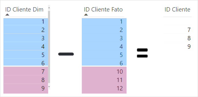
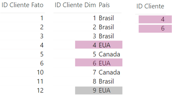
We have the following tables:

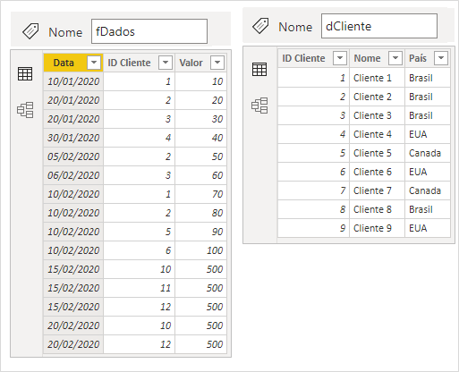
The fDados table is our fact table and the dCliente is our dimension table. Note that not all ID Cliente (Customer ID) in the fact table are found in the dimension table and vice versa.

INTERSECT function

We’ll create a physical table (via DAX) called Intersecção (Intersection) in Modeling -> New table:

Intersecção =
INTERSECT ( VALUES ( dCliente[ID Cliente] ), VALUES ( fDados[ID Cliente] ) )

When placing the ID Cliente column of this new table we created (Intersecção) in a visual, we will see that the result will be exactly those 6 ID’s (from one to 6):

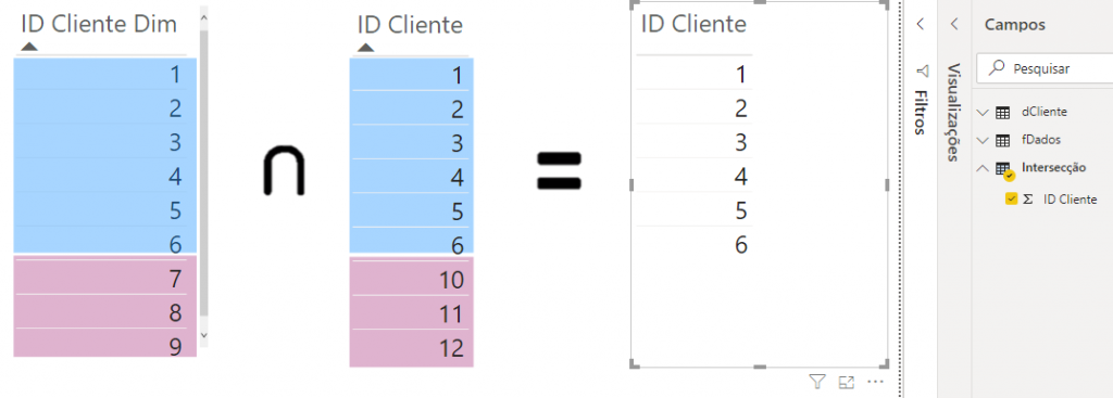
Note that I had to select the Don’t Summarize option to show all the ID’s, otherwise PBI would sum the ID’s.

In short, what we did was to represent this painted area of these two sets:

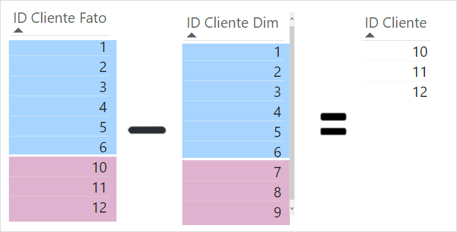
EXCEPT function

Now, what we will do is find the ID’s that exist in the dCliente table but not in the fDados table, okay?

Exceção Dim -> Ft =
EXCEPT ( VALUES ( dCliente[ID Cliente] ), VALUES ( fDados[ID Cliente] ) )

Note that in this case the order matters. See the result:

Doing the opposite, we have:

Exceção Ft -> Dim =
EXCEPT ( VALUES ( fDados[ID Cliente] ), VALUES ( dCliente[ID Cliente] ) )

And the result when we invert the order of the arguments in the EXCEPT function is this:

CALCULATETABLE function

Let’s say you need to find the ID of customers from the U.S.

The País (Country) column only exists in the dCliente and if we try to use the FILTER function we won’t be able to:

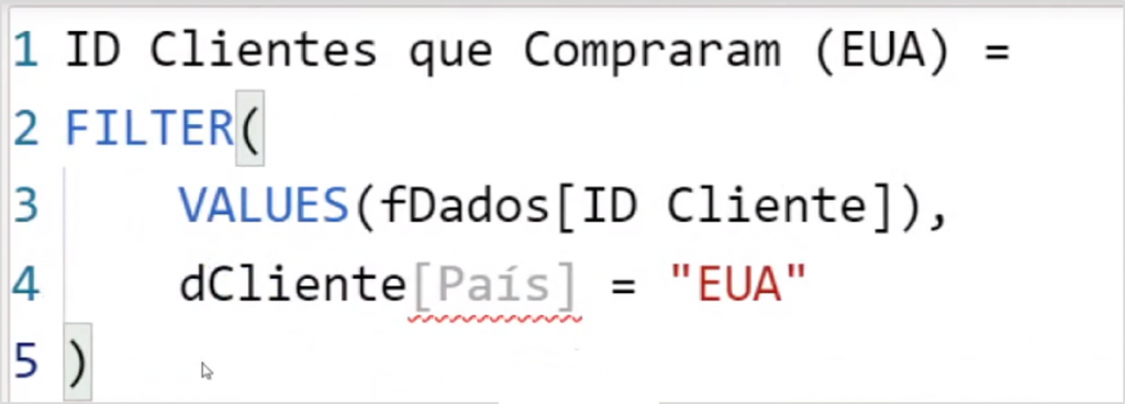
If you try to replicate this measure, an error will appear. This is because the second argument of the FILTER function must be present in the same table as the first argument. Note that we do not have a País column in the fact table so we have no other option: we will use CALCULATETABLE.

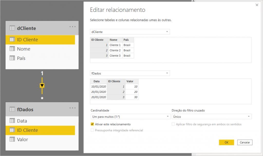
This function will allow us to filter a fact table based on a dimension table. However, before applying this function in place of FILTER, we will need to activate the relationships between the tables

Now we can apply the CALCULATETABLE function, see:

ID Clientes que Compraram (EUA) =
CALCULATETABLE ( VALUES ( fDados[ID Cliente] ), dCliente[País] = “EUA” )

Observe the result in the third table with only the ID’s that correspond to the “USA” filter. As we are filtering the fact table, it doesn’t make sense that the ID equal to 9 (in gray) appears in the result, right? Look:

Tip:
CALCULATETABLE is a function that modifies context (filters tables).
– The first argument is a table
– From the second argument onwards are the filters to be applied

Well, let’s move to the examples using a complete database.

Cases about Customers

Double Event

Our goal is to find the number of customers who have purchased two specific products – it is about working with a double event.

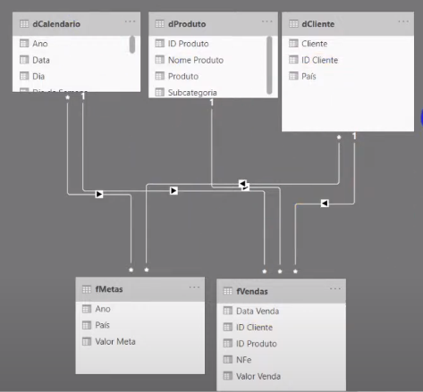
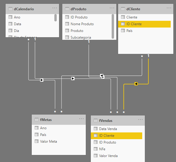
Our model is the classic one – Star schema with dimensions table for customer (dCliente), product (dProduto) and date (dCalendario) and a fact table with information on sales (fVendas). Our database has data from January 2017 to April 2019. See the model with the relationships:

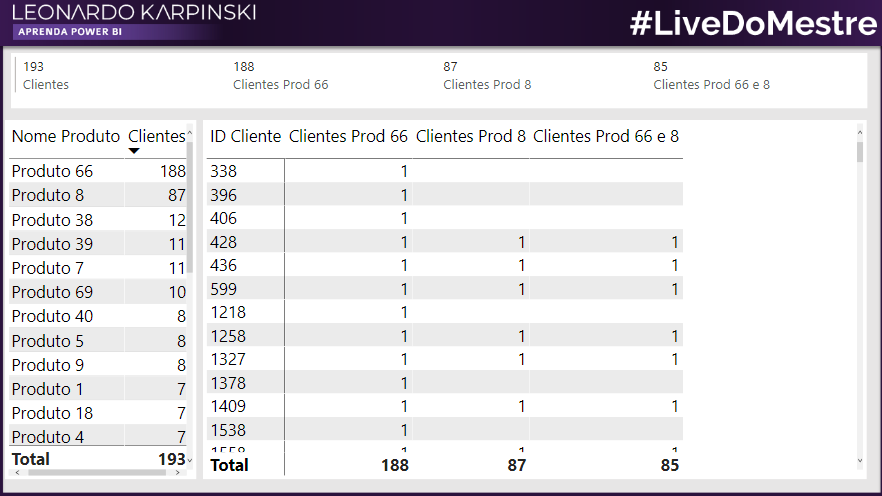
We also have the number of customers who bought each product and put these values ​​in a table using the DISTINCTCOUNT () function – in a measure called Clientes (Customers).

We will have then: a Card with the measure Clientes, a table with the Name of the product (Nome do produto) and Clientes and beside it, another table with the ID Cliente (from the table dCliente).

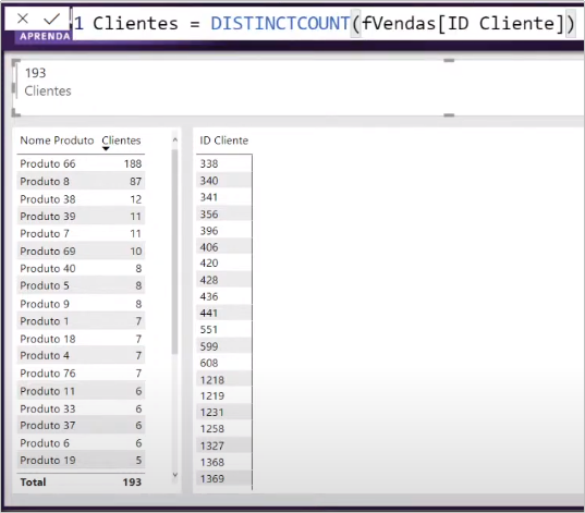
Our first challenge is to identify how many (and which) customers have purchased a particular product – Product 66.

Let’s do this using the CALCULATE function:

Clientes Prod 66 =
VAR vClientesProd66 =
    CALCULATE ( [Clientes], dProduto[ID Produto] = 66 )
RETURN
    vClientesProd66

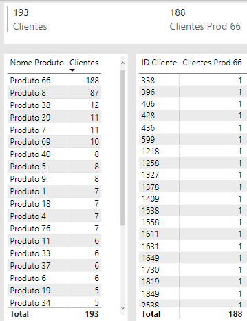
Alright! We did it, see:

It gets complicated when we add one more event: I also want to know how many (and which) customers bought Product 8. Let’s try two options:

Using “&&”:

Nao_da_certo Prod 66 e 8 (E) =
VAR vClientesProd66_8 =
    CALCULATE ( [Clientes], dProduto[ID Produto] = 66 && dProduto[ID Produto] = 8 )
RETURN
    vClientesProd66_8

Using “||”:

Nao_da_certo Prod 66 e 8 (E) =
VAR vClientesProd66_8 =
    CALCULATE ( [Clientes], dProduto[ID Produto] = 66 || dProduto[ID Produto] = 8 )
RETURN
    vClientesProd66_8

The result is:

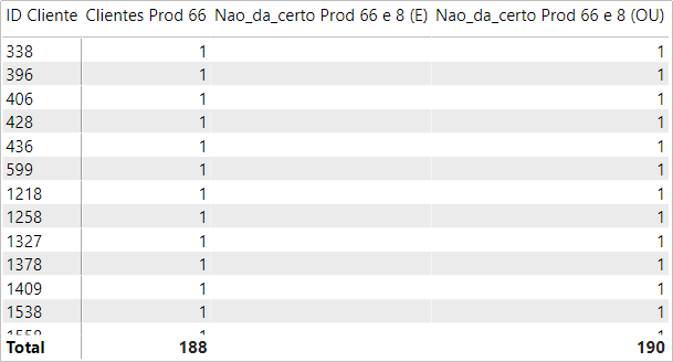
You can even try using && e || to add another condition to the filter but you will not be able to get the correct result. Shall we understand why? What I don’t recommend is:

Well, to the explanation!

Note that we had no values ​​when using “&&” (equivalent to “AND”) because it is not possible for a product to be one thing and another at the same time, right ?! It seems obvious, but you can get confused with these logical operators sometimes …

When we use “||” (equivalent to “OR”), we had a total value greater than what we found when filtering Product 66. Just look at the total values ​​in the last line of the table: 190> 188. In other words, for this case, what we got then was the Union (sum) of the ID Cliente who purchased Product 66 or Product 8. So, these two alternatives (AND / OR in the Calculate filter) don’t apply to what we want (the intersection).

Let’s repeat what we did for Product 8:

Clientes Prod 8 =
VAR vClientesProd8 =
    CALCULATE ( [Clientes], dProduto[ID Produto] = 8 )
RETURN
    vClientesProd8

Well, now let’s use those functions you learned, INTERSECT and CALCULATETABLE:

Clientes Prod 66 e 8 =
VAR vClientesProd66 =
    CALCULATETABLE ( VALUES ( fVendas[ID Cliente] ), dProduto[ID Produto] = 66 )
VAR vClientesProd8 =
    CALCULATETABLE ( VALUES ( fVendas[ID Cliente] ), dProduto[ID Produto] = 8 )
VAR vClientesAmbos =
    INTERSECT ( vClientesProd66, vClientesProd8 )
RETURN
    COUNTROWS ( vClientesAmbos )

Perfect, right ?! Check the following table:

Let’s move to our next challenge!

Recurrence

Let’s say you need to calculate how many and which customers bought in the current and previous month, that is, you want to get recurring customers. You also need to know how many customers stopped buying on each month.

Recurring customers

Our first measure will be Clientes Recorrentes 1M and to build it you will need to create some variables:

Clientes Recorrentes 1M =
VAR vClientesAtuais =
    VALUES ( fVendas[ID Cliente] )
VAR vClientesPM =
    CALCULATETABLE (
        VALUES ( fVendas[ID Cliente] ),
        PREVIOUSMONTH ( dCalendario[Data] )
    )
VAR vClientesRecorrentes =
    INTERSECT ( vClientesAtuais, vClientesPM )
RETURN
    COUNTROWS ( vClientesRecorrentes )

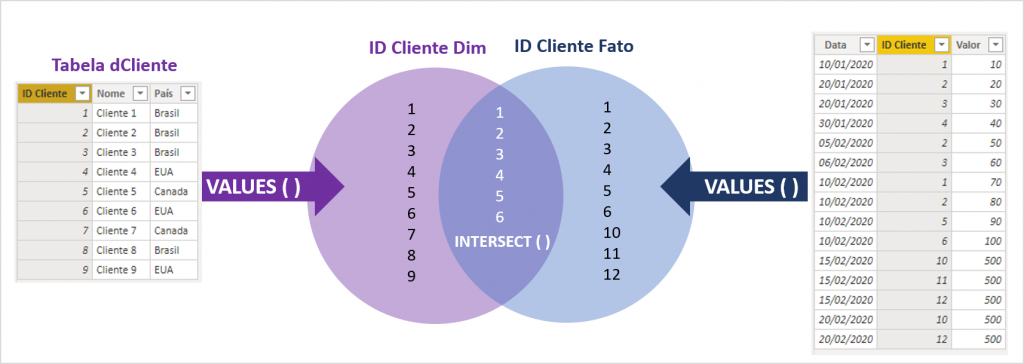
We created the variable vClientesAtuais to obtain the current customers table and this is achieved by using the VALUES function for the ID Cliente column on the fact table.

We also created the vClientesPM variable (PM from “Previous Month” – last month) to find customers who bought in the previous month. Note that the second argument of CALCULATETABLE is the PREVIOUSMONTH function to ‘go back’ a month in the dCalendario table.

Lost Customers

To find lost customers we will do the same thing. We will copy the Clientes Recorrentes 1M measure and rename it to Clientes Perdidos 1M and make some small changes:

Clientes Perdidos 1M =
VAR vClientesAtuais =
    VALUES ( fVendas[ID Cliente] )
VAR vClientesPM =
    CALCULATETABLE (
        VALUES ( fVendas[ID Cliente] ),
        PREVIOUSMONTH ( dCalendario[Data] )
    )
VAR vClientesRecorrentes =
    EXCEPT ( vClientesPM, vClientesAtuais )
RETURN
    COUNTROWS ( vClientesRecorrentes )

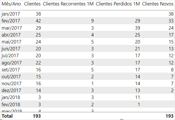
Note that we had to change the INTERSECT function to EXCEPT and also reverse the order of the arguments. Let’s see how these two measures look in the table?

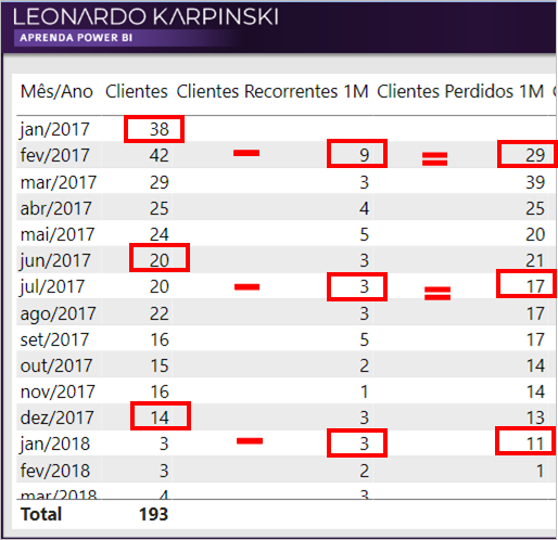
The first value in the Clientes Perdidos 1M column (value 29) represents the number of customers who bought in Jan / 2017 but didn’t buy in Feb / 2017. Notice in the above image that we highlighted how to do the ‘real test’ to check if the values ​​are correct.

Well, all set right ?! You can now create multiple metrics to analyze your customer portfolio!

You may be wondering: “How about new customers?”

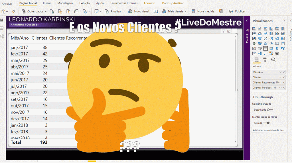
It will be our next challenge!

New customers

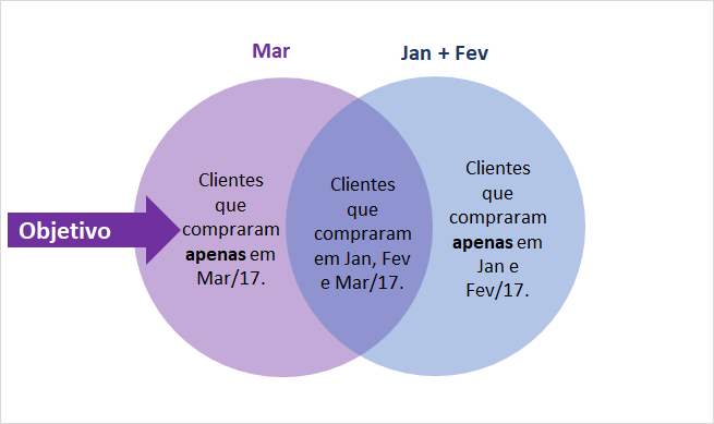
Our goal is to find, for example, in March, how many customers bought only in that month, that is, who did not buy in January or February – in the year 2017. Remember that our data starts in 2017?

The measure will be called Clientes Novos and will look like this:

Clientes Novos =
VAR vDataInicial =
    MIN ( dCalendario[Data] )
VAR vClientesAtuais =
    VALUES ( fVendas[ID Cliente] )
VAR vClientesAntigos =
    CALCULATETABLE (
        VALUES ( fVendas[ID Cliente] ),
        FILTER ( ALL ( dCalendario ), dCalendario[Data] < vDataInicial )
    )
VAR vClientesNovos =
    EXCEPT ( vClientesAtuais, vClientesAntigos )
RETURN
    COUNTROWS ( vClientesNovos )

In short, what we did was remove the old customers from the current customers (that’s why we use EXCEPT).

Let’s explain a little bit about the reasoning behind the vClientesAnterior variable.

For a customer to be considered “new” it necessaryly cannot have bought in any other period of our database, right ?! So, to get the number of previous customers we need to look at everything that comes before the current context date.

First we need to ‘see’ all the calendar dates. And how do we achieve this ?! Using the ALL function that removes the current context, right ?! That’s why we inserted it in the first argument of the FILTER function, in the Date column of dCalendario. Understood?!

Then, we need to make sure that we only see the dates before the context starts. That is, if we only want to see customers who bought in the past – before Mar / 2017, we need to remove this month (and future dates) from that account!

The current context is given by dCalendario [Data], right ?! And the beginning of the context is given by what ?! By the minimum value! So we use MIN in the dDataInicial variable for that! This way we will be able to guarantee, row by row, that we are counting only customers who bought before Mar / 17 when using the “<” operator.

From then on it’s easy! We already know the set of current and previous customers, now we just need to extract from the Current Customers set those that are “Old” using the EXCEPT function with the arguments in that order! Think like this: today I have 5 blouses, 3 of them were bought before that month, what will remain are the blouses that I bought that month. That is, 5-3 = 2 new ones!

See how the Clientes Novos (New Customers) measure is in our table:

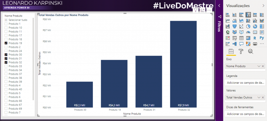
Case about Selected Products

Others

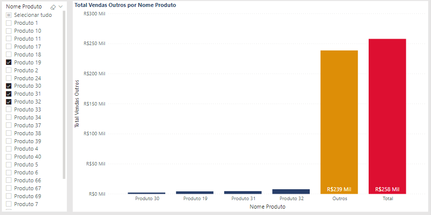
Our last task is to create an “Other” category for products not selected in the filter (data segment) and insert a Totalizer in the bar chart.

We already have the Total Vendas (Sales) measure ready:

Total Vendas =
SUM ( fVendas[Valor Venda] )

We need to create a new table via DAX:

dProdutoAux =
UNION (
    VALUES ( dProduto[Nome Produto] ),
    ROW ( “Nome Produto”, “Outros” ),
    ROW ( “Nome Produto”, “Total” )
)

This created table will have a column with all the products and two more lines (Total and Others). It will be used in the Axis of the bar chart.

We will also create a measure called Total Vendas Outros to obtain all values ​​for the unselected products.

Let’s do it in parts and at the end I will show the complete formula, ok ?! The first part:

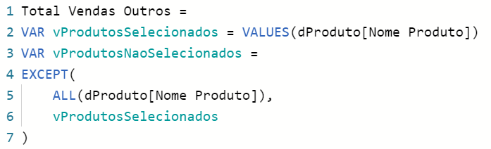
This part represents the same idea of the previous example, using EXCEPT: of all products that had sales (use of ALL in the Product table), we will remove all selected products and what will remain are the “OTHER” products.

The second part will be to obtain the Total Sales value of the selected products and for that we will need a variable called vProdutosEixo:

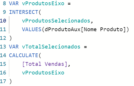
See that we need to show in the graph only the selected products. Do you remember that we created an auxiliary table called dProdutosAux? We need to intersect the values ​​(names) in this table with the selected products. And how do we do that ?! Using the INTERSECT! This function will make a “virtual relationship” between the tables.

After that, we calculate the sales value of the selected products (vTotalSelecionados). Notice that in the CALCULATE filter we insert the variable vProdutosEixo created earlier!

By applying Return on vTotalSelecionados, we can see that it worked:

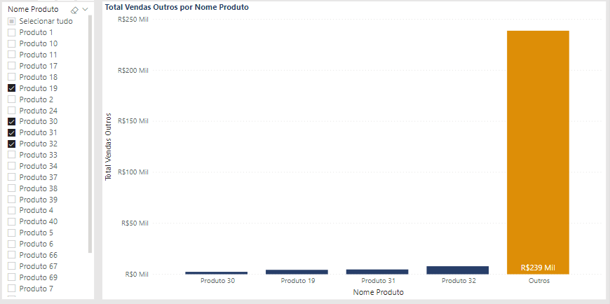
But where’s the bar with “Others”? Let’s do this!

Creating the variable vTotalOutros …

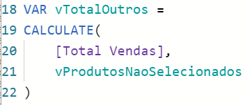
Now notice that the CALCULATE filter is vProdutosNaoSelecionados that we created on part 1.

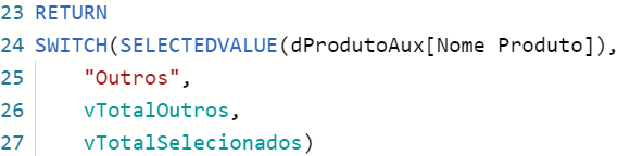
We need to indicate PBI which value to use for each axis item so we will need SELECTEDVALUE function to indicate the context and the SWITCH function to choose which variable to use. If my context (X-axis value) is Outros (Others) I need to use the vTotalOutros measure, otherwise we will use the vTotalSelecionados.

The chart looks like this:

Total

Finally, we’ll calculate Total de Vendas Fixo (Total Fixed Sales) in a separate measure:

Total Vendas Fixo =
CALCULATE ( [Total Vendas], ALL ( dProduto ) )

The use of ALL you already know: it’s for any filter applied.

Everything good so far?

We will return to our Total Vendas Outros measure to add another pair of arguments in the SWITCH function:

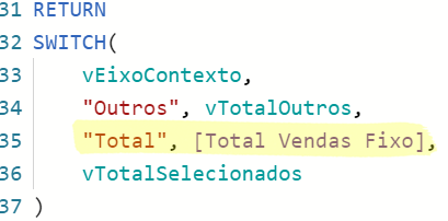
Ready! Now it’s perfect, see:

As promised, here’s the complete formula for the variable Total Vendas Outros:

Total Vendas Outros =
VAR vProdutosSelecionados =
    VALUES ( dProduto[Nome Produto] )
VAR vProdutosNaoSelecionados =
    EXCEPT ( ALL ( dProduto[Nome Produto] ), vProdutosSelecionados )
VAR vProdutosEixo =
    INTERSECT ( vProdutosSelecionados, VALUES ( dProdutoAux[Nome Produto] ) )
VAR vTotalSelecionados =
    CALCULATE ( [Total Vendas], vProdutosEixo )
VAR vTotalOutros =
    CALCULATE ( [Total Vendas], vProdutosNaoSelecionados )
RETURN
    VAR vTotalOutros =
        CALCULATE ( [Total Vendas], vProdutosNaoSelecionados )
    VAR vEixoContexto =
        SELECTEDVALUE ( dProdutoAux[Nome Produto] )
    RETURN
        SWITCH (
            vEixoContexto,
            “Outros”, vTotalOutros,
            “Total”, [Total Vendas Fixo],
            vTotalSelecionados
        )

The only change we made was to leave SELECTEDVALUE in a separate variable called vEixoContexto, ok ?!

See?! With a little effort and intermediate knowledge in DAX we were able to solve our challenge without workarounds!

Physical and virtual relationships

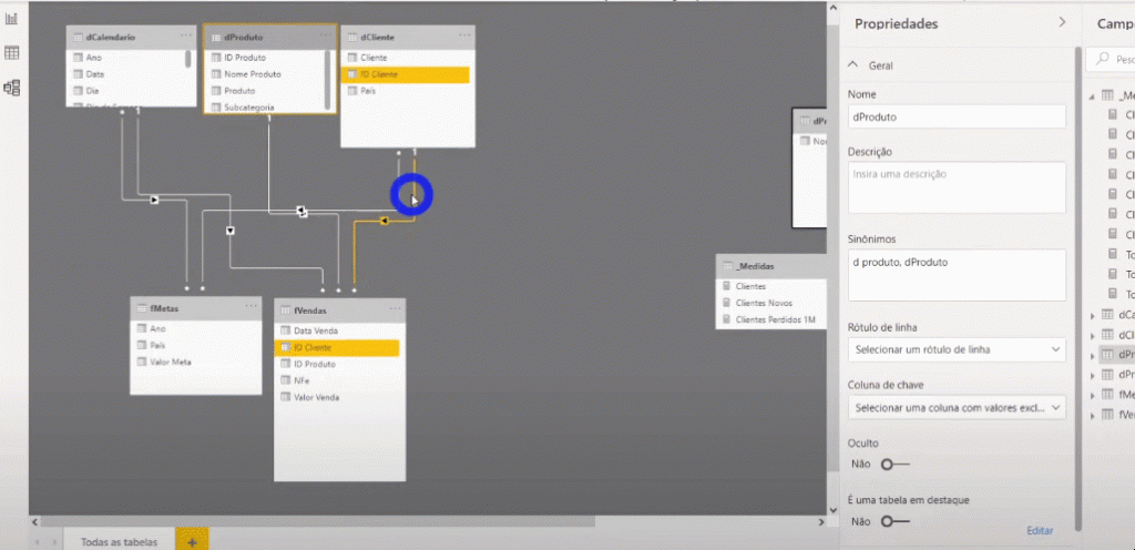
Note that there is already a physical relationship between dCliente and fVendas:

Let’s assume that for some reason you need to have this relationship disabled.

If we have a table with the ID Cliente and Total Vendas, what will happen to it when we disable the relationship from the above image?

Problem: The Total Vendas value will remain constant for each row in the table.

How can we make the value correct in the table ?!

Solution 1: Use USERELATIONSHIP!
Solution 2: Use IN!
Solution 3: Use INTERSECT!
Solution 4: Use TREATAS!

USERELATIONSHIP application

Solution 1 would then be to create this measure:

Total Vendas USERELATIONSHIP =
CALCULATE (
    [Total Vendas],
    USERELATIONSHIP ( dCliente[ID Cliente], fVendas[ID Cliente] )
)

Then the table would correctly show the sales value:

The question is:

Is this relationship Physical or Virtual?

IT’S PHYSICAL!

It is physical because there is a relationship between dCliente and fVendas but it is inactive. When we use USERELATIONSHIP we temporarily ‘activate’ this relationship for measure use.

But what if you can’t afford not having a physical relationship (active or inactive)? In this case we will be able to use any of the other solutions – 2, 3 and 4. We will start with solution 2: use of IN!

IN application

We will create a measure called Total Vendas Relac. Virtual and we will modify it according to the solution to be shown, ok ?!

Using IN:

Total Vendas Relac. Virtual =
VAR vClientes =
    VALUES ( dClienteRLS[ID Cliente] )
VAR vClientesFiltradosIN =
    FILTER ( VALUES ( fVendas[ID Cliente] ), fVendas[ID Cliente] IN vClientes )
RETURN
    CALCULATE ( [Total Vendas], vClientesFiltradosIN )

Result with the use of IN:

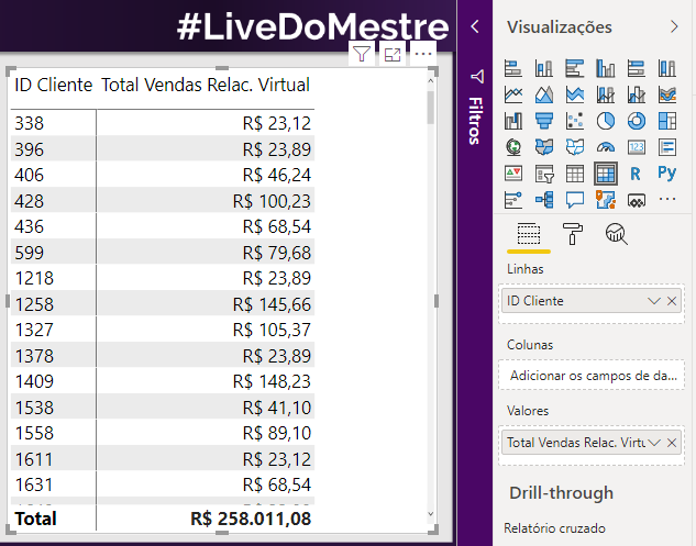
INTERSECT application

For solution 3 (using INTERSECT), we have:

Total Vendas Relac. Virtual =
VAR vClientes =
    VALUES ( dClienteRLS[ID Cliente] )
VAR vClientesFiltradosINTERSECT =
    INTERSECT ( VALUES ( fVendas[ID Cliente] ), vClientes )
RETURN
    CALCULATE ( [Total Vendas], vClientesFiltradosINTERSECT )

You can read this formula like this: The customers of the dimension table (vClientes) are filtering the fact table. The result in the table will be exactly the same in all solutions, ok ?!

TREATAS application

The last solution (4) will be through TREATAS. The formula is a little different:

Total Vendas Relac. Virtual =
VAR vClientes =
    VALUES ( dClienteRLS[ID Cliente] )
VAR vClientesFiltradosTREATAS =
    TREATAS ( vClientes, fVendas[ID Cliente] )
RETURN
    CALCULATE ( [Total Vendas], vClientesFiltradosTREATAS )

The first argument of TREATAS will be the table that will filter and then the column that will be filtered.

Of the 4 options if you need to choose the most performatic one always choose the physical relationship (use of USERELATIONSHIP). It is the option that will return the values ​​faster on large databases!

Now if you can’t physically do this in your model, the order of performance (from best to worst) for virtual relationships is: TREATS >> INTERSECT >> IN.

Phew, now it’s over! We did a lot today, huh ?!

I hope you enjoyed the content! Whenever you need, it will be available here to consult, ok ?!

Regards,
Leonardo.