BLOG DOS
INCOMPARÁVEIS

Hey, everyone! How is it going?!

Have you ever considered using the Python + Power Bi combination in your projects? Are you interested in making future sales forecasts or creating custom visuals with Python scripts? Mario Filho will help us with these tasks and give us some really cool tips! He is a Data Scientist and a specialist in Machine Learning – and has won prizes in several international competitions on this subject.

Today’s content was based on Youtube Live # 15 Master Power BI, ok ?!

Dica:
On Mario Filho’s website, you will find links to his classes, ebook, podcasts, courses, and more! Click on the link to check it out: https://www.mariofilho.com/

After all, what is Python?

Like Java, C, R, Python is a “general purpose” programming language – you can do almost anything with it.

The difference between Python and R is that, since Python has a very easy and simple syntax to write, it ended up being adopted by the Data Science, Machine Learning, and scientific community in general. Because of this, several ML libraries were developed for Data Science and therefore Python ended up replacing R in many cases.

Why did you choose Python over R and why is Python better than R?

Point of contention! There is no such thing as Python being better than R! We must make it clear that R is a statistical language. You will find in R the most exotic there are in statistics! And definitely for that purpose, R ends up being better than Python.

When you think about a project as a whole and the integrations you may have with other software or languages ​​it’s much easier to do this with Python. It works as a bridge between some languages, for example, you can call a C code within your Python code and still have a good performance.

So for this simplicity of syntax and ease of integration with other languages ​​and software, Python has been gaining more and more prominence in the community.

How and where can I use Python in Power BI?

Some possibilities of using Python in Power BI we identified:

1. Import data sources that are not available or don’t perform really well in PBI (web scrapping, non-relational databases, etc.);
2. Apply Power Query data transformations;
3. Incorporate Machine Learning into your base;
4. Create custom visual elements with Python libraries.

We will cover in detail items 3 and 4, which are the most used applications! Let’s go through step by step so you can perform the PBI + Python integration. Ready ?! Let’s do this!

Step by Step to use Python

We need to install Python! Follow these steps:

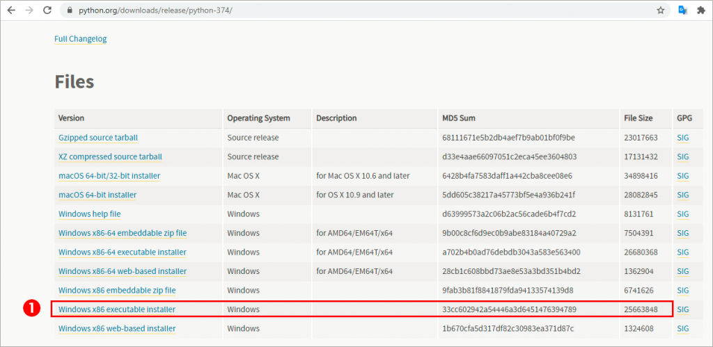
1. Download the Python 3.7 file through the website and install it. The executable file to download can be found on https://www.python.org/downloads/release/python-374/

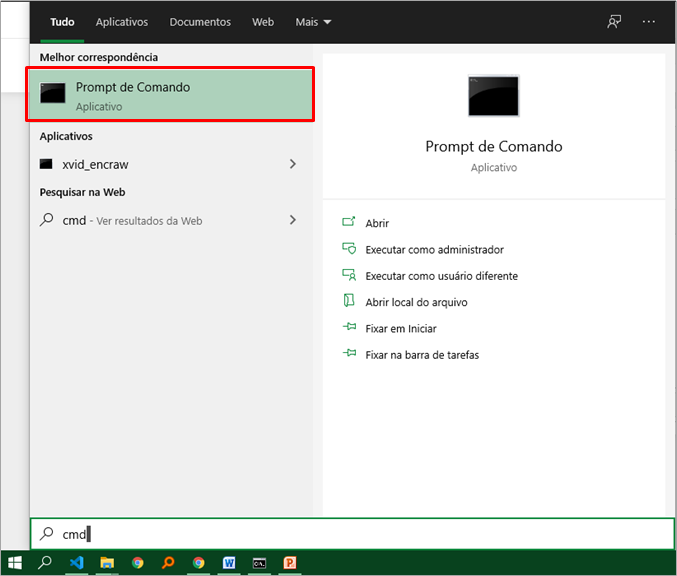
2.  Open CMD (command prompt):

Just type “cmd” in the Windows search bar as follow:

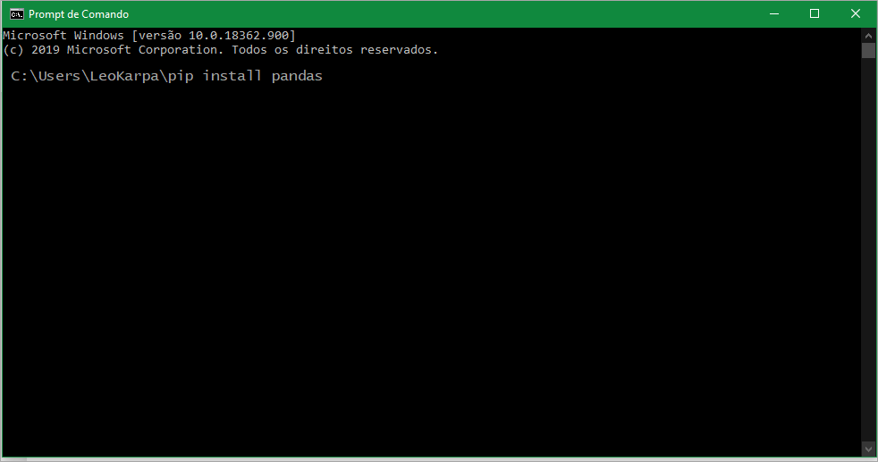
3. Install the following libraries by typing in the CMD window:
pip install pandas
pip install xlrd
pip install matplotlib
pip install scikit-learn
pip instal plotnine
pip install seaborn
pip install notebook

Type each line above one at a time. After typing the first line, hit enter. Wait for the installation to complete and proceed to the next one.

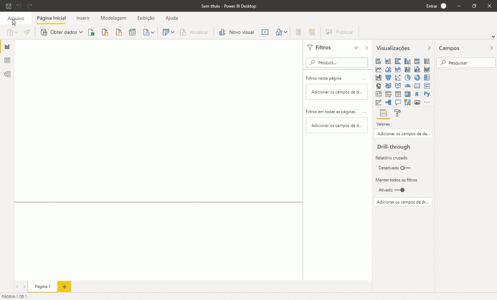
4. In Power BI Desktop, disable the option “Store data sets using the enhanced metadata format” in Preview features. Check below:

5. If Power BI does not automatically identify the Python directory, you must add it manually:

Steps:
File → Options and Settings → Python Scripting → Detected Python home directories:

Challenge 1: Sales Forecast

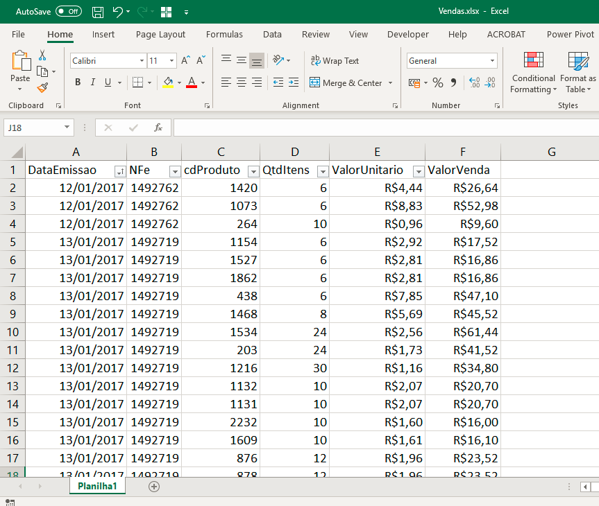
Data base

Our scenario has the following database: an Excel file with columns for Invoice Issue Date (DataEmissao), Invoice (NFe), Product code (cdProduto), Sold items quantity (QtdItens), the Unit value of each product (ValorUnitario), and Sale value (ValorVenda). Check below

Writing in Python

In this section, we will show you the code line by line and describe what was done in each of them. In the end, I will provide the complete code (for copy and paste), ok ?!:

During the Youtube Live, Mario used the Jupyter lab to run Python commands line by line. We are going to replicate the procedure using the Jupyter notebook, okay? In the end, it turns out to the same! Don’t worry about installing Jupyter Notebook on your computer now, the goal at this point is to understand what each line of code will do with our data.

An important aspect is that the Vendas.xlsx file must be in the same directory as Jupyter Notebook in order to test the code, ok ?!

First, we start with the import command for the library we are going to use:

Python Command:

import pandas as pd

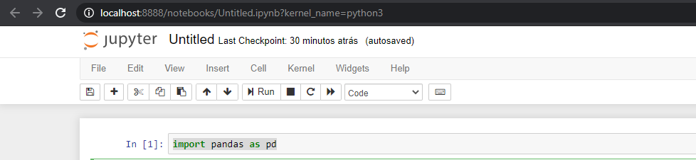
Just type the above command in the first cell and click Run.

Note that when we use “as pd” it is as if we are giving a nickname to our library (usually, they are small words and represent the library we are going to use in the commands below). You will notice in the next line that we will use “pd” to indicate from which library we are using a given function.

Ah, this line has no outputs so we can move on to the next command.

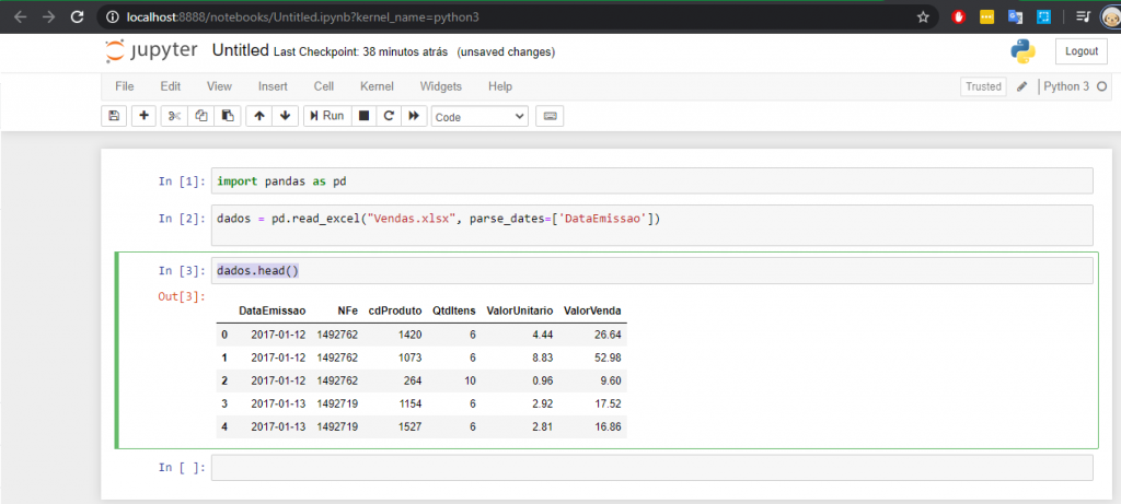
Python command:

dados = pd.read_excel("Vendas.xlsx", parse_dates=['DataEmissao'])

This command also has no outputs. It only serves to load the data – that Excel file (our database).

A good tip is to always insert the parse_dates argument (even if it’s not mandatory) since Python will not always recognize the Dates column automatically, ok ?!

Tip:
Tell Python what your file’s Date column is by using parse_dates as an argument to the read_excel or read_csv function (if your file is .csv) when using Pandas.

Next line! Type the command below:

Python command:

dados.head()

If you leave the argument empty as it is in the above code, we will be able to see the first 5 lines of our loaded data. But you can change it to 10, 15, 100 if you want to see more lines, ok ?! This command generates an output, look:

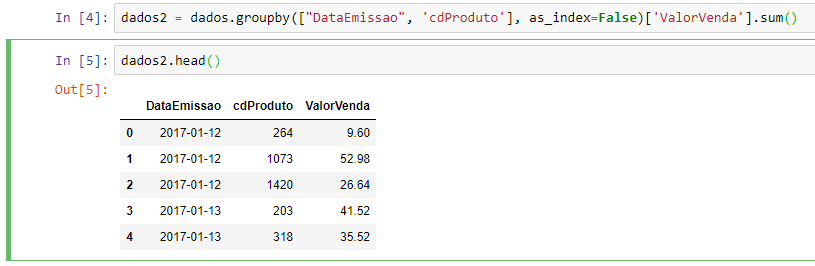
Well, our goal is to make a daily sales forecast but we know that there is more than one invoice issued per day, right ?! With this in mind, we will need to group our data by product and date (columns cdProduto and DataEmissao). With that, we will have a record for each date and each product, ok ?!

Python command: 

dados2 = dados.groupby(["DataEmissao", 'cdProduto'], as_index=False)['ValorVenda'].sum()

See that the name of the data frame (data2) is different from the name of the data frame of our original database (data), ok ?! We are using our original table (data) and performing a grouping based on two columns.

When using the groupby function we need the name of the columns that will be unique, in this case, there are two: “DataEmissao” and “cdProduto”. Which means, this pair of values ​​will be unique in each row.

Ah, the argument as_index = False is important! If we don’t insert it, we’ll have to work with the panda index and that will make our model a bit complicated.

What about the “SalesValue” column? It will be aggregated (added) for each of the unique values ​​that appear, that’s why the sum () function for that column.

Looking at the result from dados2.head() we have:

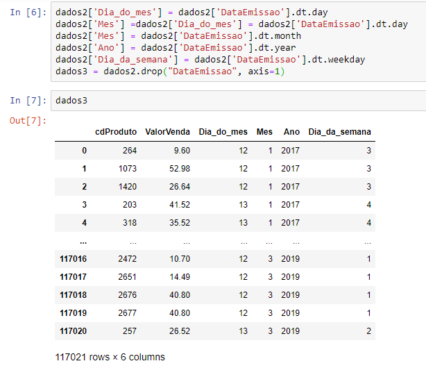
Now, we need to separate that date into some components and then remove it. See that the commands below are very intuitive:

Python command:

dados2['Dia_do_mes'] = dados2['DataEmissao'].dt.day
dados2['Mes'] =dados2['Dia_do_mes'] = dados2['DataEmissao'].dt.day
dados2['Mes'] = dados2['DataEmissao'].dt.month
dados2['Ano'] = dados2['DataEmissao'].dt.year
dados2['Dia_da_semana'] = dados2['DataEmissao'].dt.weekday
dados3 = dados2.drop("DataEmissao", axis=1)

As we have already shown Python that our date column is DataEmissao, it will be possible to easily find the day, month, year, and day of the week from that column using the above functions (dt.month, dt.year, etc). In the end, the drop function will delete the column “DataEmissao” after all we already have all the components we need.

Let’s check how it looks? If we just type the name of the data frame we created (data3), we can see the following in Out [7]:

This step is important because it will help our model to understand the seasonality of sales.

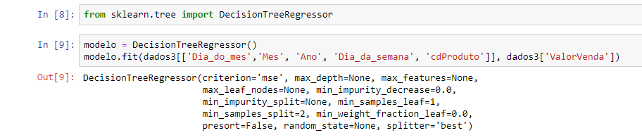
Now, we will need the Scikit-learn library. It is the most popular Python Machine Learning library.

We are working with a Machine Learning model called supervised. Basically, you use the input variables and the target (what you want to predict) as input. The model will try to find patterns that will relate these variables and try to predict new targets. And to do that, we will use a decision tree.

The first thing we are going to do is identify the days, months, days of the week that are most predictive – that stand out the most. We can provide as an example the month of December that since, in general, it has more sales of panettone if we are talking about a store that sells these types of products. Or, if we are talking about a costume shop, February is the month that stands out the most – which means, sales increase at this time because of the carnival, right ?! These are the rules that the model will try to find in our database, always with the objective of predicting the future sales value.

Python command:

from sklearn.tree import DecisionTreeRegressor
modelo = DecisionTreeRegressor()
modelo.fit(dados3[['Dia_do_mes','Mes', 'Ano', 'Dia_da_semana', 'cdProduto']], dados3['ValorVenda'])

After the import command, we create the object called model and we will use the decision tree to make a regression, hence the name DecisionTreeRegressor ().

In the line below we see the fit method. It’s the method for the model to find/learn the rules we mentioned, based on the informed columns. So this method will look at all the data that we entered as an argument and look for the best rule that predicts the value of the sale for each day and product and, finally, it will store these found rules. See the Out [9] below:

You must be thinking:

– Got it, Mario! The model has already learned these rules and showed them on the screen. Now, how to make the model predict sales on future dates?

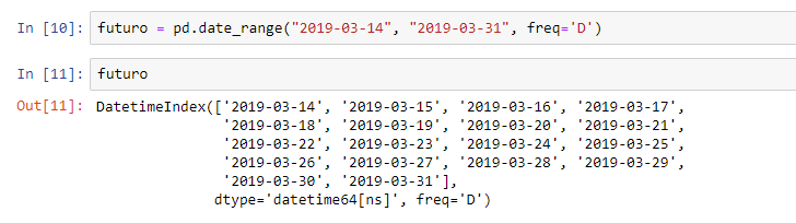
We will first need to use a Pandas function called date_range. Through this function, we will define the future date range. The syntax is quite simple:

Python command:

futuro = pd.date_range("2019-03-14", "2019-03-31", freq='D')

This function will create a sequence of dates. The first argument will be the first date equal to 2019-03-14. We set this date because it is the date after the last sales date in our base – in image 9 we see that the last sale occurred on 2019-03-13. The next argument represents the end date of the interval. And, as a third argument, we insert freq = ‘D’ because we want a frequency in days, ok ?!

When typing the name of this object (futuro), we will see the result:

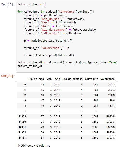
With these created dates, the next step is to create those date decompositions (similar to what we did for DataEmissao: day, month, year, day of the week) and associate each date line with a product code (cdProduto). The code looks like this:

Python command:

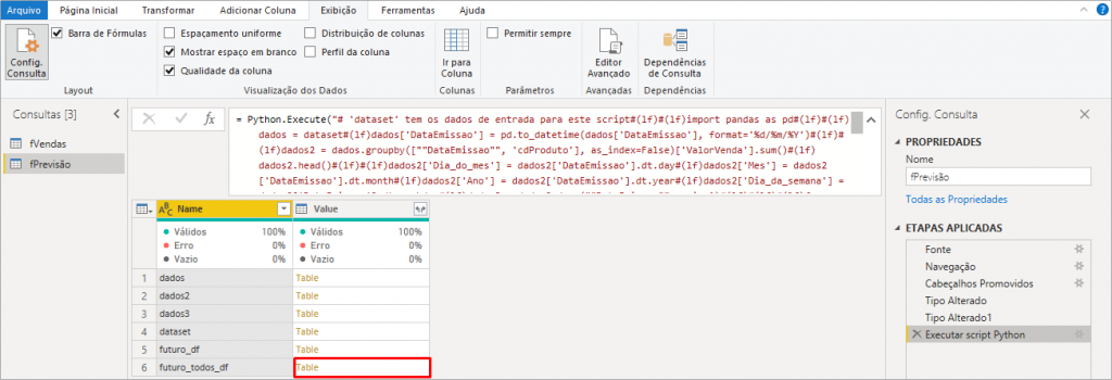
futuro_todos = []
for cdProduto in dados3['cdProduto'].unique():
     futuro_df = pd.DataFrame()
     futuro_df['Dia_do_mes'] = futuro.day
     futuro_df['Mes'] = futuro.month
     futuro_df['Ano'] = futuro.year
     futuro_df['Dia_da_semana'] = futuro.weekday
     futuro_df['cdProduto'] = cdProduto

p = modelo.predict(futuro_df)

futuro_df['ValorVenda'] = p
futuro_todos.append(futuro_df)

futuro_todos_df = pd.concat(futuro_todos, ignore_index=True)
futuro_todos_df.head()

Note that the order of decomposition of the future date was the same as we did for DataEmissao, ok ?!

See that we also use the predict function which is responsible for generating sales forecasts for each future day (which we specify in that date range) and for each product.

The append function will save all those data frames we created in the list futuro_todos. See that we created an empty list at the beginning of the code when we wrote the syntax futuro_todos = []. This append is for adding items to that list.

In the end, we use the concat function that will take these data frames and join them into one. See the result below:

Did you like it?! Few lines of code and we were able to obtain sales forecast values! We went through the code very quickly but the idea is to have an overview of what is possible to do with Python + Power Bi, ok ?! If you need to go deeper into the topic, take a look at Mario Filho’s website because there is a lot of cool stuff there!

The complete code looks like this (you’ll need it for the next step):

import pandas as pd

dados = pd.read_excel("Vendas.xlsx", parse_dates=['DataEmissao'])

dados2 = dados.groupby(["DataEmissao", 'cdProduto'], as_index=False)['ValorVenda'].sum()
dados2.head()

dados2['Dia_do_mes'] = dados2['DataEmissao'].dt.day
dados2['Mes'] = dados2['DataEmissao'].dt.month
dados2['Ano'] = dados2['DataEmissao'].dt.year
dados2['Dia_da_semana'] = dados2['DataEmissao'].dt.weekday
dados3 = dados2.drop("DataEmissao", axis=1)


from sklearn.tree import DecisionTreeRegressor

modelo = DecisionTreeRegressor()
modelo.fit(dados3[['Dia_do_mes','Mes', 'Ano', 'Dia_da_semana', 'cdProduto']], dados3['ValorVenda'])


futuro = pd.date_range("2019-03-14", "2019-03-31", freq='D')

futuro_todos = []

for cdProduto in dados3['cdProduto'].unique():
    futuro_df = pd.DataFrame()
    futuro_df['Dia_do_mes'] = futuro.day
    futuro_df['Mes'] = futuro.month
    futuro_df['Ano'] = futuro.year
    futuro_df['Dia_da_semana'] = futuro.weekday
    futuro_df['cdProduto'] = cdProduto

    p = modelo.predict(futuro_df)

    futuro_df['ValorVenda'] = p

    futuro_todos.append(futuro_df)

futuro_todos_df = pd.concat(futuro_todos, ignore_index=True)
futuro_todos_df.head()

Moving on to Power BI …

Adding the forecast script to Power BI

Import the Vendas.xlsx file into Power BI and rename the query in the query editor to fVendas (‘f’ is for Fact Table). Duplicate this query and rename it to fPrevisão.

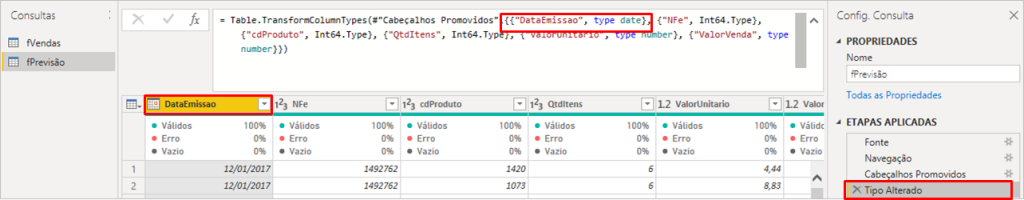
Note that Power BI will automatically apply a data type transformation step in the DataEmissao column, but we don’t want this because the Python date format is different from the PBI’s. See the transformation applied automatically:

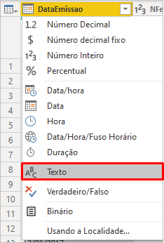
To correct, just change the type to text (inserting a new step – or editing the current one):

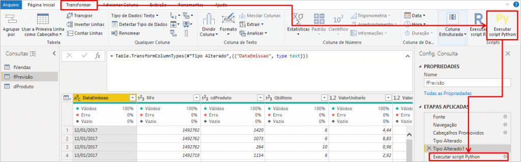
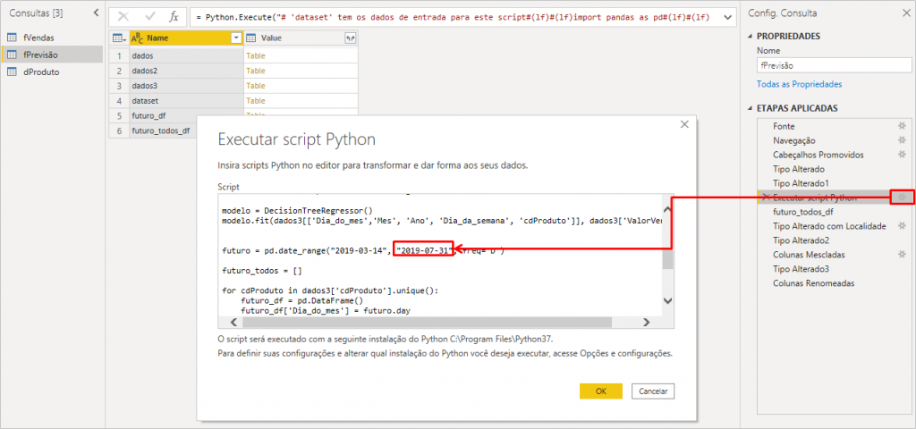
Now let’s add our Python Script by clicking on the Run Python Script button:

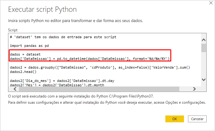
In the next window, insert the complete code above displayer replacing the line “data = …” as indicated below:

Remove this snippet of the complete code:
data = pd.read_excel ("Vendas.xlsx", parse_dates = ['DataEmissao'])

Add this snippet in place of the removed snippet:
data = dataset
data ['DataEmissao'] = pd.to_datetime (data ['DataEmissao'], format = '% d /% m /% Y')

See how it looks:

After clicking OK, it will take a while for the PBI to execute the Python script.

It is always good to point out that it is preferable that you run the script outside the PBI and throw the result of the script into a database, for example – so that the BI team will be able to connect directly to the database to extract this data. I mean:

Always the right tool for the right problem!

MARIO FILHO

We are showing something that is possible to do in PBI but if you have an outside structure to run this script and insert the data into a database, it is better, ok ?!

In short: the ideal scenario is that the processing (ML model creation and training) takes place outside the PBI. There is no tool that’s good at everything! Power Bi is great for simple ETL, DAX / data modeling, not to mention visuals … For ML models creation and training as well as making complex ETL’s, no! Look at the time it took the PBI to load the tables and run the Python Script!

Is everything clear ?! Let’s move on…

Well, we will see that Power Query will show the list of tables within our script and we should only expand futuro_todos_df:

After expanding the table by clicking on the Table name in yellow (referring to line 6 in the above image), we will have the futuro_todos_df step applied:

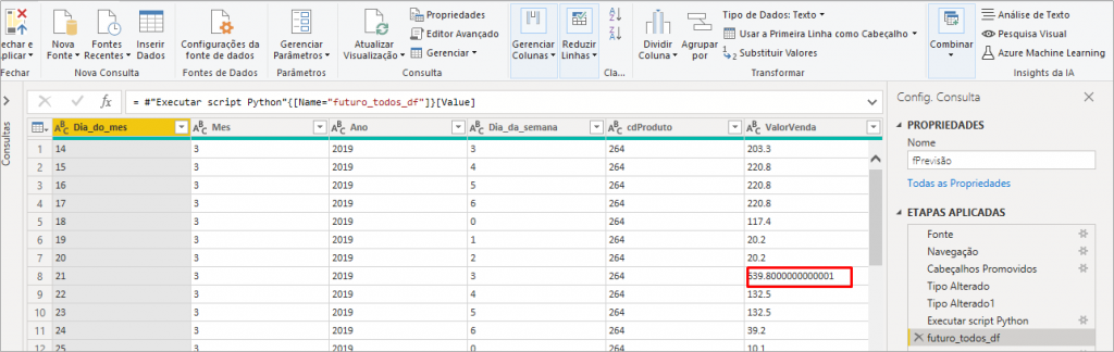
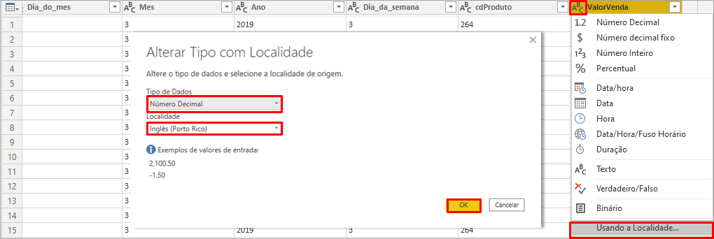
Analyzing the result after the expansion of futuro_todos_df, if PBI has applied a transformation step “Type changed2”, exclude this step leaving only the steps up to the one shown in the above image. Note that in line 8 the value of the SalesValue column has several decimal places. This may happen when PBI reads a number as text. We will correct this by modifying the changed type using Locale, like this:

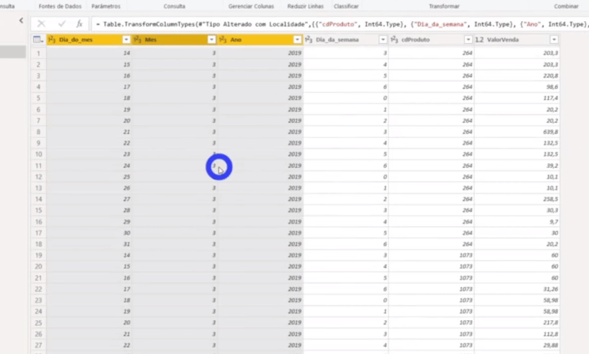
Check if the columns Month_Day, Month, Year, and Weekday_Date are formatted as a Whole number and if they are not, change to Decimal number.

We don’t have a date column in that table, right ?! We need to build it and we will do it by merging columns. Just select the Columns Day, Month, and Year with the CTRL key activated; right-click and select the Merge columns option. See more details below:

Don’t forget to change the column Forecast Date to Date type, ok ?!

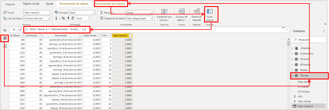
Ah, we forgot the dProduto table! Creating this table will be easy. Just duplicate fVendas, delete all columns except the cdProduto column (which must be formatted as Whole number) and remove duplicates. Check it out:

It’s very important to be cautious and check if the columns will make relationships are formatted with the same numeric type, ok ?! So dates must be in date format, product code as a whole number, and values ​​(sales) as decimal numbers in every table.

Now, just click Close and apply in Power Query!

Creating the dCalendar table with DAX

Let’s create a dCalendar table to list all the dates in our model. To do this, just go to Modeling and New Table.

In the formula bar type:

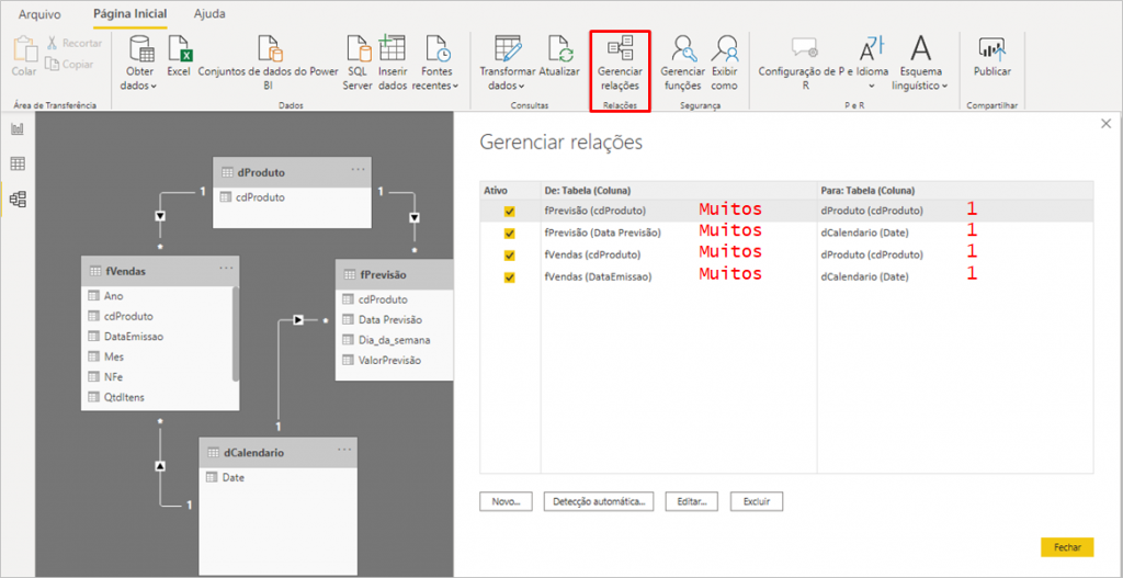
When configuring the relationships between tables, we will have the following:

Visual

It’s time to create our first chart!

Our aim is to show the possibilities that we have of integrating Python with Power BI, so we won’t be worrying about the design and beauty of graphs, ok ?!

Ah, a detail before adding our first chart: I edited the date range that the model will predict by editing the Run Python script step. Feel free to change the range the way you prefer, ok ?!

Our chart looks like this:

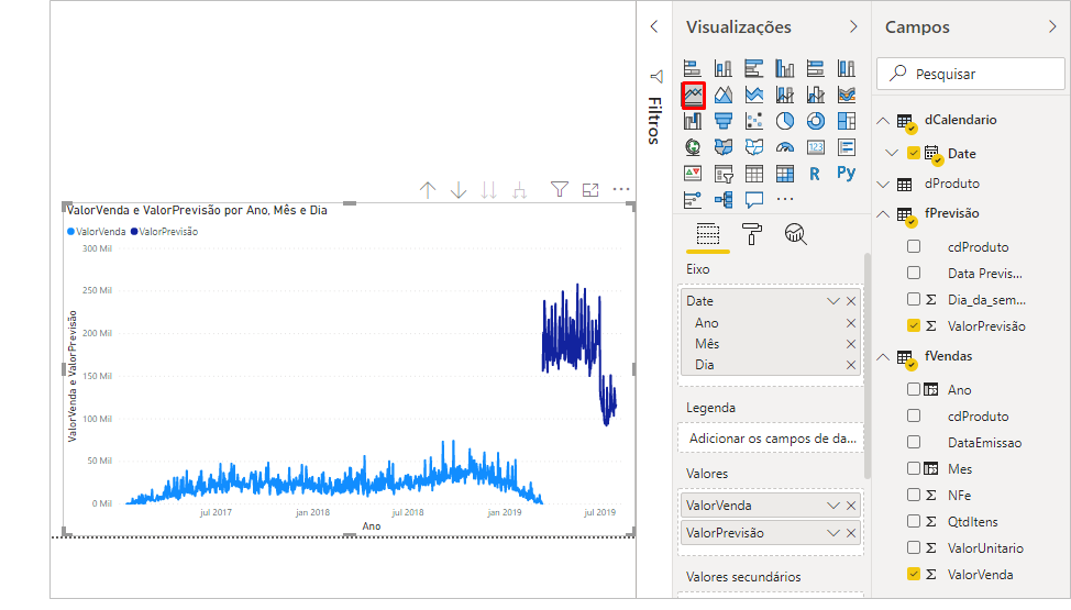
The chart we created is the Line Chart. You may be wondering about the behavior of the forecast values ​​curve (in darker blue). We did this example very quickly for demonstration purposes and we have several techniques that we could implement in the script to improve this model. However, if we filter product by product, the values ​​start to make a little more sense, see:

Now, let’s move on to the next challenge: creating a visual with Python!

Challenge 2: Creating visuals with Python

Database

Our database consists of an Excel table with CHURN data and has the following columns:

Import this table into Power BI and go to Reports (where we will create our charts).

Example 1

The first thing we will do is click on the Python Visual. See that a Script Editor will appear below the page:

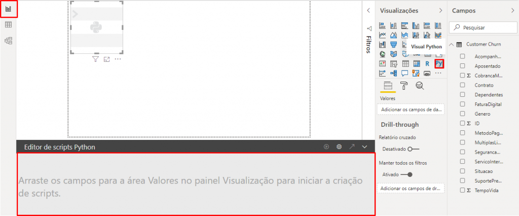
When we add the columns in this visual, the editor will automatically add some rows, check it out:

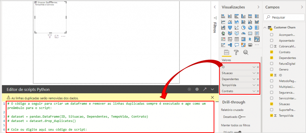
Now we will add this code (just 4 lines) below line 6 in the Python Script Editor:

Python command:

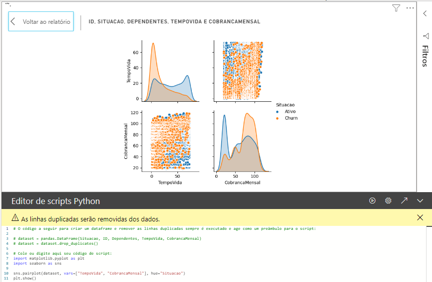
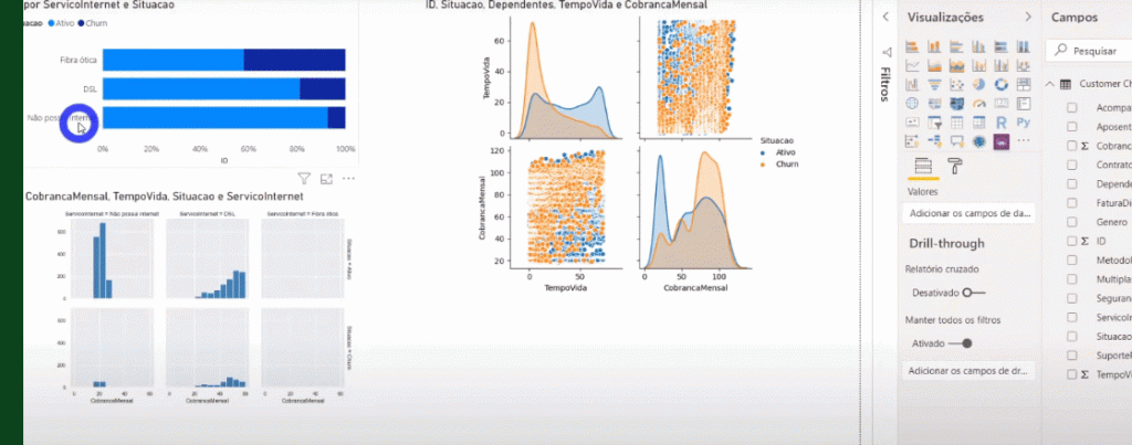
import matplotlib.pyplot as plt
import seaborn as sns

sns.pairplot(dataset, vars=["TempoVida", "CobrancaMensal"], hue="Situacao")
plt.show()

After applying this code in the editor and clicking the “play” button, we will have this look:

Let’s move to another example!

Example 2

This time we will use the columns: ID, MonthlyBilling, LifeTime, Status, and InternetService. Copy and paste the code below into the editor:

Python command:

import numpy as np
import seaborn as sns
import matplotlib.pyplot as plt
sns.set(style="darkgrid")

tips = dataset
g = sns.FacetGrid(tips, row="Situacao", col="ServicoInternet", margin_titles=True)
bins = np.linspace(0, 60, 13)
g.map(plt.hist, "CobrancaMensal", color="steelblue", bins=bins)
plt.show()

For this visual, I used the code from this site: https://seaborn.pydata.org/examples/faceted_histogram.html and made the necessary adjustments. Here’s what I modified from the original code:

Tip:
I used the site https://seaborn.pydata.org/examples/index.html to search the code for each visual (and their respective libraries).

Now, look how cool! We were able to add a native Power BI visual and filter the Python visual!

See below that if we add a bar graph, for example, and select a bar, we will be able to ‘filter’ Python graphs (but the opposite is not possible):

Remember that for R codes it is the same thing, only the syntax changes – which is specific to each language, ok ?!

So we finished today’s content! We were able to show in detail how the Python + Power BI integration works in two applications.

I hope you enjoyed! See you!

Regards,
Leonardo!