If you work with large transactional databases, suffer from slow dashboards and think that DirectQuery (DQ) is the solution to your problems then you are in the right place! We’ll explain why you should avoid this connection type in Power BI!
Power BI has 3 data source connection types: Import, DirectQuery and LiveConnection.
Just to give you an overview … LiveConnection is a dynamic connection to an Analysis Services model (SSAS or AAS). It is as performative as Import because it uses the same background engine (tabular model).
Today’s battle is between Import and DirectQuery, ok ?!

Scenario
Imagine the following situation: your data is in a SQL Server database. You need to connect to that database in order to build your PBI report, okay ?!
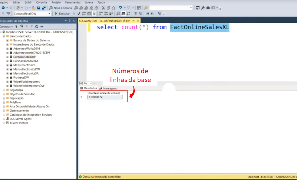
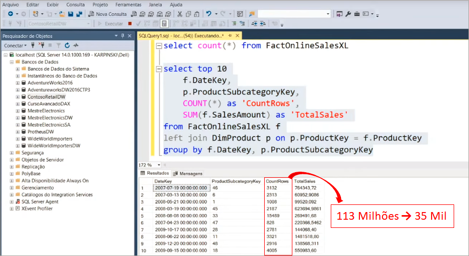
We will make a connection in the ContosoRetailDW database and use the FactOnlineSalesXL table. Take a look at the database size using Microsoft SQL Server Management Studio:
In PBI Desktop, as soon as you select SQL Server Database, these two connection options will appear:
If you haven’t watched our Youtube Live # 26 you may be like this:

Calm down! We will show the difference between these two connection types and at by the end of this article you will have no further doubts about it!
Import
In this type of connection, the data is imported into PBI Desktop and stored in your computer’s memory. When the report is published, the data will be stored in the memory of the Microsoft server (the Cloud one).
This connection type guarantees an excellent performance during data analysis because when importing them, PBI performs an important compression in each column of the model. Then, PBI saves each compressed column in a different space in memory. That is, the data is cached in the memory of the computer on which you are developing the report.
This has two consequences: the .pbix file will become large and the data refresh will take longer to be completed. But watch out: this shouldn’t be an excuse to use DirectQuery! We’ll soon see how to get around these problems!
Performance using Import
Let’s perform the first test by selecting the Import connection type.
After importing the FactOnlineSalesXL table into PBI Desktop it will take a little time to load all the lines … Be patient and have a coffee while you wait … As soon as the loading is finished, save the .pbix file, ok ?! Ah, when saving is complete, the file size is 586 MB!

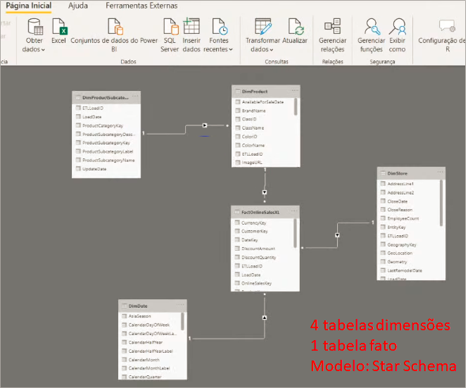
The model for our example is the most basic: Star schema.
I left a blank page and another one with two visuals in the report to be able to analyze the performance more consistently (we will do the same with Direct Query).
We will use the Performance Analyzer to measure the processing time required to create or refresh the report elements started as a result of any user interaction that results in the execution of a query.
To use it, just go to Display → Performance Analyzer. Leave the Blank page selected, click Start recording and switch to the second page (Import). Look:
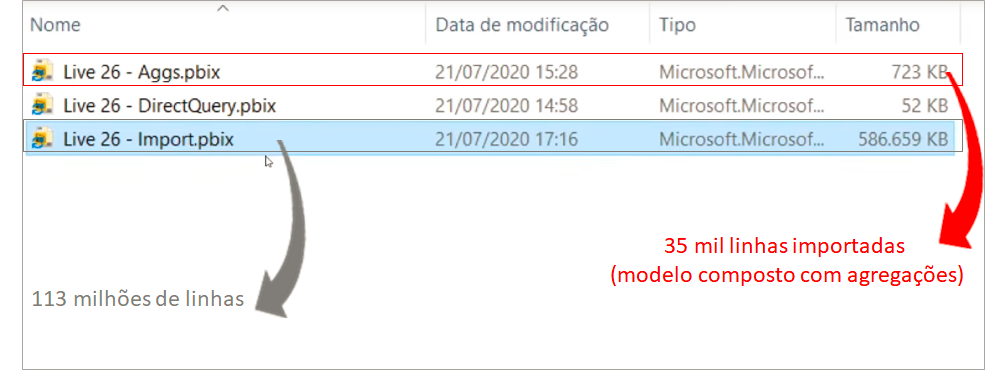
Remember those 113 million lines? It only took about 3 seconds in total to process everything. Super fast! However when saving the report, the .pbix file size was 586 Mb!
DirectQuery
Unlike the Import mode, when using DirectQuery you will not be importing the data into the .pbix file, that is, they will remain at the data source (server that contains the connected database) and you will perform queries in that data source during the data analysis.
This connection type works like this: if you apply a filter on a report graph, this will be translated into a query. This query will be sent to your data source, processed and finally the data will return refreshed to your PBI. Therefore, all pressure and load will be under the responsibility of the server where your data is stored.
The main advantage of the connection via DQ is that the data will always be refreshed, since for each interaction PBI will look for the data directly at the source. Another advantage is that the .pbix file will be smaller since no data will be stored – only the metadata is stored in the file.
This connection type presents low performance for the end user (who will use your report) and in addition, if the database you connect to is being used for other purposes there may be competition on your server and impact not only the data analysis on Power BI, but also the use by other users who depend on that server and possibly even bring it down. Can you imagine the tragedy ?!
In summary, the main aspects that often lead people to use DirectQuery are:
- Big data volume – where Import mode may not be capable of handling;
- Need for real-time data
Performance using DirectQuery
Let’s connect to our database using the SQL Server database.
The .pbix file has the same pages as the test we did previously (using Import), ok?
We’ll use the Performance Analyzer to measure the processing time again. This time prepare yourself psychologically because it will take time to process! See the SQL Server memory consumption as we process (in this example the “server” is my own machine):
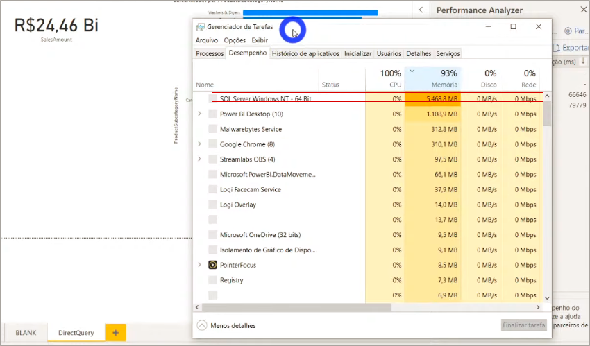
Oh, just for the record: when we save the .pbix file, its size is 52 Kb!
The total processing time was approximately 1 minute (in Import mode it was 3 seconds, remember?). You may be considering this time ‘reasonable’ but remember: we only had 1 bar chart and a card on this page of the report! Can you imagine a complete panel ?! The user will give up using the report because it won’t handle to wait that long for each analysis / interaction.
Did you realize that the assumption “I have a large database” is not enough to exclusively use DirectQuery as a connection mode?
Solutions
Before we talk about solutions, we need to make the following clear:
It is essential that the connection is made in a Data warehouse and not in the production database!
Especially when we think of DirectQuery! Otherwise you will be competing with the production database at all times. As it was already mentioned: you may bring the server down !
A very common complaint:
My report is slow, what can it be?
You will first need to identify where the slowness is. The options are:
- In Power Query and data refreshing
- In the data model (.pbix is very large – above 500 MB)
- Dax measures (we’ll talk about DAX performance in another article)
Now I ask you: which of these cases is the most critical?
If you answered 1, let’s think together … When you update the data on PBI, at what time do you usually do that ?! When you are developing? When users are making analysis? I don’t think so! Generally refreshes are scheduled to occur during non-business hours, such as at dawn, on weekends … So no problem if this update takes 30 or 40 minutes, okay ?!
Remember: you must think about the report end user!
Golden rule: Power Bi needs to be fast for those who will analyze the data, and not for you who is developing it!
Calm down! I won’t just say that and run away! There are indeed ways to make development fast!
For development to be fast, you need to ensure two things:
- Good performance machine: above 8GB of RAM and SSD disk
- Import only a sample of the data during development (filter rows)
I’m sure tip 2 will change your life going forward! We will do this through a feature called Incremental refresh.
Our goal is to solve two problems: slow development and delay in updating.
Incremental Refresh
Before showing the step by step you need to know that to use this feature you must have at least a PRO account.
Parameters creation
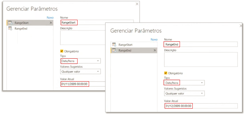
We will need to create two parameters: RangeStart and RangeEnd. To do this, open Power Query → Home → Manage Parameters → New Parameter and then fill in the fields as shown in the image below:
Filter fact table rows
The next step is to filter the fact table rows (it’s the table with 113 million rows, remember ?!) using these parameters we have just defined. We must filter the DataKey column on the FactOnlineSalesXL table, see:
After applying this filter, our fact table was reduced to 8 million rows. The x.pnix file size was reduced from 586 MB to 31 MB!
Setting the Incremental Refresh
Now we need to indicate to Power BI that we want to refresh only the last two months of the fact table and not the entire database. To set the incremental refresh, just right-click on any table in the Fields panel and follow the step by step:
You may be wondering why we created those two fixed parameters (RangeStart and RangeEnd) … They are fixed on those start and end dates (2 months duration) for development purposes. RangeStart and RangeEnd will be dynamic when we publish the report on PBI Online!
Reminder:
Power BI Desktop is your development environment. Never import all rows when developing, it’s an absurd waste of resources and a huge waste of time. The database only needs to be complete for the published report on the online service.
If you have any questions about this, visit this link to read the Microsoft documentation: https://docs.microsoft.com/en-us/power-bi/admin/service-premium-incremental-refresh
For now we solved “slow development” and “delay in updating” problem because we reduced the size of the .pbix file and configured the PBI to refresh only the last two months.
However, for the end user – who will access the published report on PBI Online, we still have that five hundred and a few MB file (full database), and the model will still not be as performatic for.

So, let’s solve the poor performance problem in the online service with the following tips:
- Import only tables and columns that are really necessary for the analysis: start small and then grow according to the client’s real needs.
- Use the Star schema model, with descriptive fields only in dimensions. Ex: product names in the fact table and in the dimension table.
Reminder:
The main enemy of performance is the number of columns and its cardinality (number of different values).
To know which columns and table to optimize, you must use VertiPaq Analyzer (which is inside DAX Studio).
Identifying columns and tables to be optmized
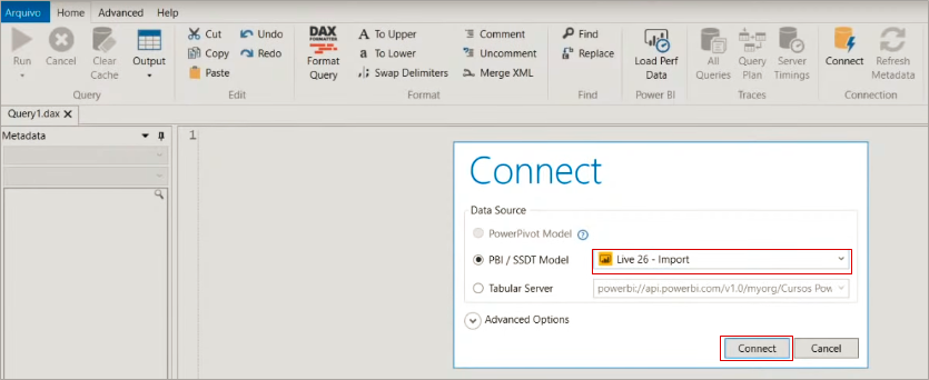
DAX Studio is a free tool and is available for download at this link. As soon as you open the program, this browser window will appear so you can select the .pbix file you want to analyze (it must be open):
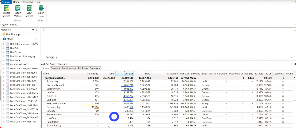
By clicking on the Advanced tab and selecting View Metrics you will be able to see exactly how much memory each column in your model consumes! See that in our example the OnlineSalesKey column consumes 30.68% of the database (% DB). It is a primary key on our fact table and since we don’t need this column in our model, we can delete it without concern!
Let’s also delete the SalesOrderLineNumber column. When we save this .pbix file we will see that it’s size went from 31 MB to 6 MB! In Power BI the behavior will be the same: size reduction!
Tip:
You should never take the fact table primary key to the PBI! If you want to count rows you can use measures (you don’t need a column numbering the rows in the fact table)!
After deleting these two columns, if you click ViewMetrics again that table will be refreshed. Now the biggest column in our model is ProductKey. But we can’t exclude this because we need it in the relationship between the fact and dimension table, ok ?!
After doing all of this, your model may still be slow.
– What now, Leo ?!

Aggregations in composite models
This functionality is available to PRO users (it doesn’t require Premium capability).
First, to find out if this solution applies to you, answer the following question:
Do you really need to analyze everything at the SKU level, by the client’s registered number, per day, etc.?
Proceed if your answer is “no”. If you answered “yes”, take a look at this solution nonetheless to have in mind how to work with aggregations in PBI when you need it!
Our goal is to summarize the fact tables (by product category, or customer segment, for example). By doing this we will be reducing the data volume and consequently we will have a considerable performance gain in the queries.
The main ways to create aggregate tables are:
- Directly in Power Query
- Using a query in PBI
- Bringing an aggregated view
- Bringing an aggregated table
We will create a composite model bringing the Aggregate Table using Import and the Detailed Table using DirectQuery and finally, we will configure the Aggregations in Power BI Desktop!
Aggregations directly in Power Query
To start creating a composite model that makes use of Aggregations, bring everything up in DirectQuery first.
In this example we will work on the same file used to show the connection mode via DirectQuery. In Power Query we will duplicate the query FactOnlineSalesXL and rename it to FactAgrPQ, ok ?! This will be our aggregate table!
To transform it into an aggregate table, just go to Group by and define how you want to group the columns:
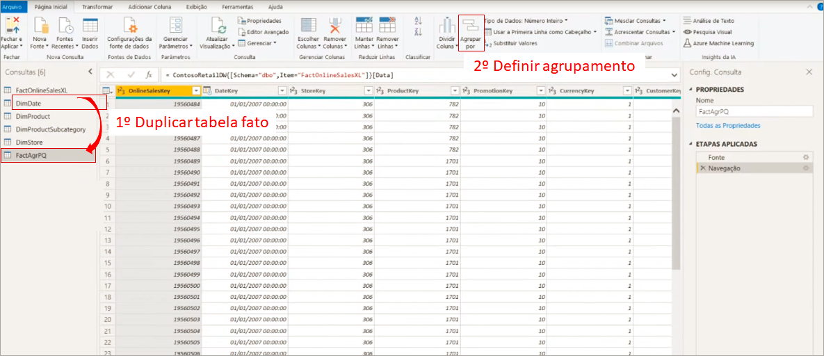
In our example, the FactOnlineSalesXL table doesn’t have a product subcategory, so we would have to merge the product table before creating this aggregate table in order to be able to group by product subcategory. So, let’s try another approach: using aggregate view in the SQL database.
Aggregate View
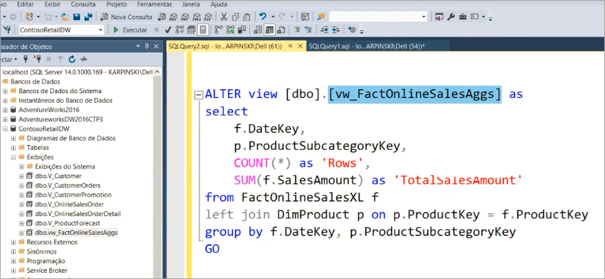
To use this option, you must create an aggregate view in Microsoft SQL Server Management Studio. See the reduction in data volume that will be applied when we group by product subcategory:
The view created will be called vw_FactOnlineSalesAggs, see:
Now just connect this view to PBI Desktop! To make it faster we will now import via DirecQuery (but in the end we will change the storage mode to Import, ok ?!).
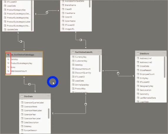
So, just to remember: the FactOnlineSalesXL table is the “original” (complete) fact table and the vw_FactOnlineSalesAggs table is our grouped table (only 35 thousand rows).
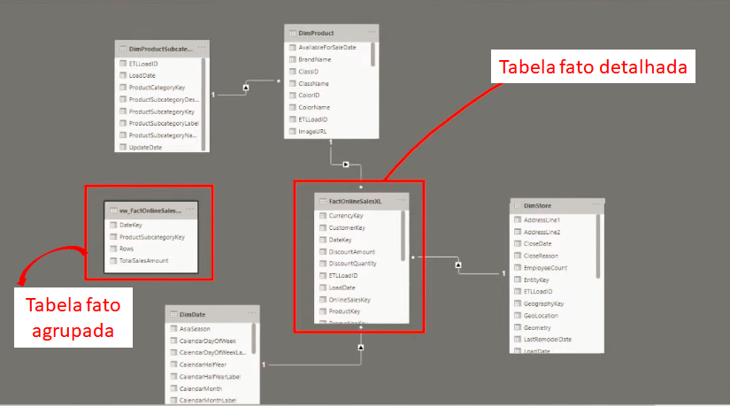
We need to relate the new tables with those already in the model, see:
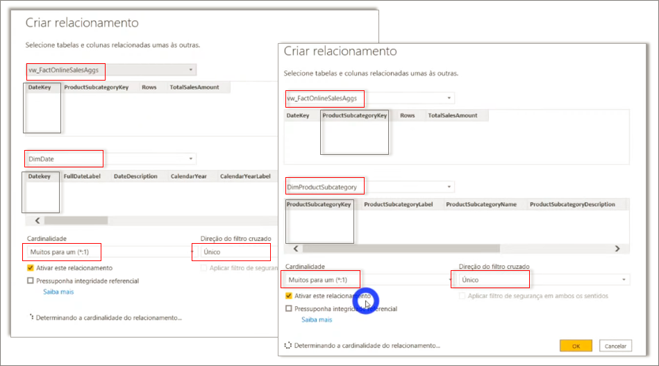
You will notice that we will now have the Snow Flake model – it’s the most practical way of relating our grouped table in the model.
Now comes the trick! Remember when I said that we were connecting to the aggregate table via DirectQuery just to make things faster (to be faster) and then we would switch to Import mode? This is what we’ll do next:
When you change the storage mode to Import, a message appears suggesting that you set the DimProductSubCategory and DimDate tables to Dual mode.
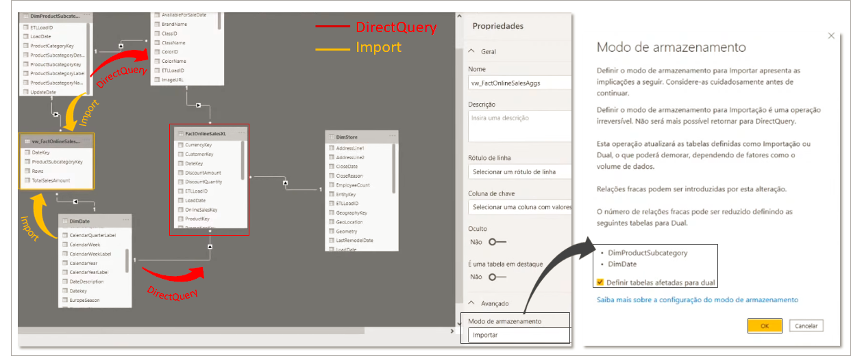
If we analyze these two tables we see that in one direction we are going to a table stored via DirectQuery and in the opposite direction via Import. By clicking OK on this message, we will set these dimension tables to Dual to reduce the number of weak relationships in the data set and improve performance.
Managing aggregations
We will basically do the same as we did in SQL. Now PBI will automatically make that choice according to the settings we define. To do this, just right-click on the grouped fact table (vw_FactOnlineSalesAggs) and then on Manage aggregations. See the final setting:
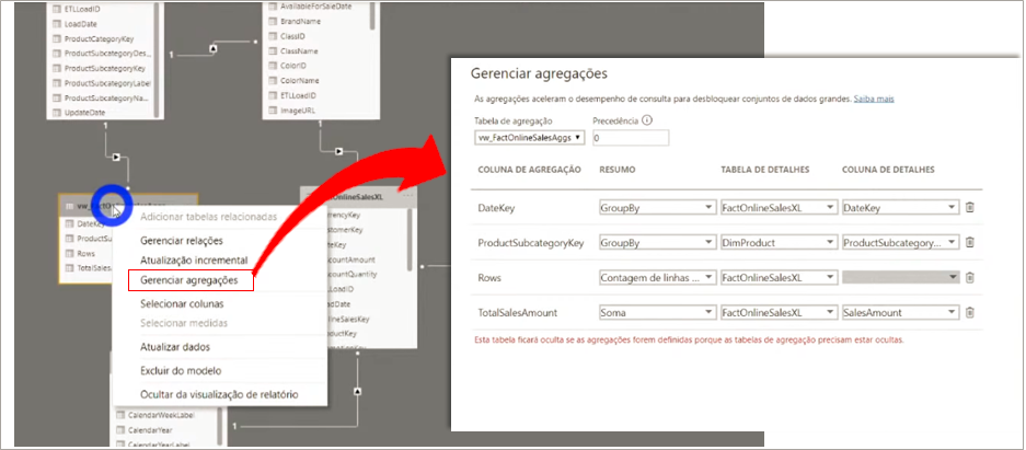
Note that the PBI will automatically hide this grouped table, after all we already know when to use it according to the rules we have set, right ?! The user doesn’t need to know that it exists!
Note the the .pbix files sizes side by side:
Performance using composite model
We will also use the Perfomance Analyzer, just as we did with the previous files to check the processing time.
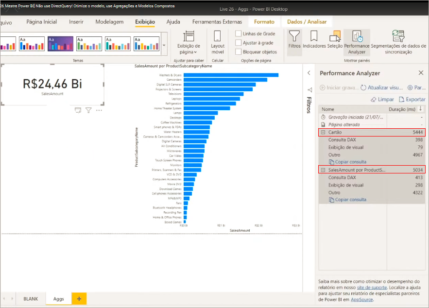
It’s important to mention: whenever you create a measure use the detailed fact table. Never use the aggregate table to create DAX measures, okay ?!
If you are curious to see what is going on behind each process in this Performance Analyzer panel, click on Copy Query to see the query that Power Bi makes and paste into some text editor. Here’s an example of when we show data from a table that is in Import mode on a card:
Now see an example using data from a table that has not been aggregated (DirectQuery mode):
Notice the difference between queries. See how many steps the SQL query has – this is because the data is not cached in memory, remember ?!
Working with real-time data
I don’t usually work with this type of model (and I don’t like it) but as promised I will show you how I would work with data in ‘real time’.
Our history will be fixed and we will only bring data from the last month (or the last two months) through DirecQuery. We’ll bring the rest (history) by using the Import mode. In practice, we will import the same fact table (one using Import mode and the other using DirectQuery mode) and apply different filters to each one, see:

Relate the fact tables normally (same relationships):
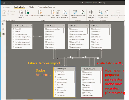
To have a visual with information from both tables, we simply create measures that add up the values of each one to obtain, for example, the total sales from the past until today.
During Live # 26 a spectator asked:
Leo, would you put parameters for the table with DQ to be on the same axis as Import’s time?
Leonardo Brito
Yes! In the table that is in DirectQuery, apply a filter in Power Query (or in the query) to bring only the previous day and back.
If you made it this far: congratulations! The content, besides being extensive, had a more technical aspect. Below we’ll consolidate the most important conclusions to finish with a flourish!
Concluions
- Do not use everything in DirectQuery, as it is slow;
- Always focus on performance in the data model, before thinking about making development light;
- To make development light, you must filter the data and work with only one slice;
- Use incremental updates to make refreshes quick;
- To make the model more performative, take as few columns and tables as possible;
- If it is still not enough, use Aggregations with composite models (Aggregated table in the Import model + Detailed table in the DirectQuery model);
- To work with real-time data, apply a filter to restrict the number of rows in DirectQuery. The rest (last) you must bring in Import mode.
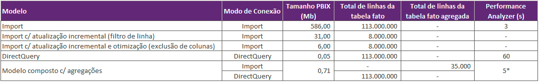
See also the summary of the tests we did:
Useful links
Microsoft recommendation on preference for using Import mode:https://docs.microsoft.com/en-us/power-bi/connect-data/desktop-directquery-about
DAX Studio Download: https://daxstudio.org/
Storage modes: https://docs.microsoft.com/en-us/power-bi/transform-model/desktop-storage-mode
We have reached the end of another article! I hope you enjoyed it! See you soon!
Regards,
Leonardo.